P2-5.2 Distribution, Mean, and Variance
Section ID:
P2-5.2Version:v2026.09.15
A distribution shows where values are concentrated and how many are there. The mean summarizes the center, and variance summarizes the spread around the mean. Two datasets can have the same mean but different distributions and variances.
Score Intervals and Counts
Grouping 10 test scores into intervals shows where the values are concentrated.
40, 45, 48, 50, 52, 55, 58, 60, 62, 90
In a histogram, the horizontal axis shows score intervals and the vertical axis shows the number of values in each interval. Here, every interval is 10 points wide. Each interval includes its left boundary, while its right boundary belongs to the next interval.
| Score interval | Scores in the interval | Count |
|---|---|---|
| 35 ≤ score < 45 | 40 | 1 |
| 45 ≤ score < 55 | 45, 48, 50, 52 | 4 |
| 55 ≤ score < 65 | 55, 58, 60, 62 | 4 |
| 65 ≤ score < 75 | None | 0 |
| 75 ≤ score < 85 | None | 0 |
| 85 ≤ score < 95 | 90 | 1 |
A score of 45 belongs to the second interval, and 55 belongs to the third. Defining the boundaries this way avoids counting the same score twice. Adding the interval counts gives 10, the original number of scores.
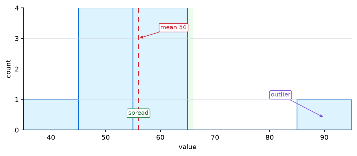
Eight of the 10 values fall between 45 inclusive and 65 exclusive; none fall between 65 inclusive and 85 exclusive. The score of 90 is separated from the other values. The red dashed line marks the mean of 56. A mean line alone cannot show empty intervals or separated scores, so the arrangement of the bars must also be read.
Data Distributions and Probability Distributions
A distribution can refer to the arrangement of observed data or to the probabilities of possible values.
| Expression | English | Working Explanation |
|---|---|---|
| data distribution | data distribution | the shape in which the values of actually observed data are arranged |
| probability distribution | probability distribution | a mathematical expression that assigns probabilities to possible values |
For example, suppose there are actually 100,000 user-age data points. If we draw them as a histogram, we are looking at the data distribution.
By contrast, if we express mathematically how likely is each possible value to appear?, that is a probability distribution.
A data distribution talks about how already collected values are arranged, while a probability distribution talks about with what probabilities possible values might occur.
They are connected, but they are not the same thing. We may look at a real data distribution and assume or estimate a probability distribution, but that does not mean the observed data itself is the complete probability distribution.
This distinction matters in AI. The distribution of training data is the shape of the data the model actually saw, while the distribution of the real world is the shape of the data the model may encounter later. If the two distributions differ, model performance may become unstable.
Calculating the Mean
The mean is the value that summarizes many values into one representative center.
Suppose there are the following values.
2, 4, 6, 8, 10
The mean is calculated by adding all values and dividing by the number of values.
Written with sigma notation, it is the following.
Sigma compresses the calculation that adds all the values. Dividing the sum by the count n gives the mean.
The mean is used very often. The reason is simple. It compresses many values into one number that can be compared. This is how we read the average response time this month, the average clicks per user, the mean loss of a batch, and the model's average accuracy.
But the mean does not tell us every feature of the data.
Same Mean, Different Spread
The mean shows the center quickly, but it can hide the shape of the values.
Suppose there are two data bundles.
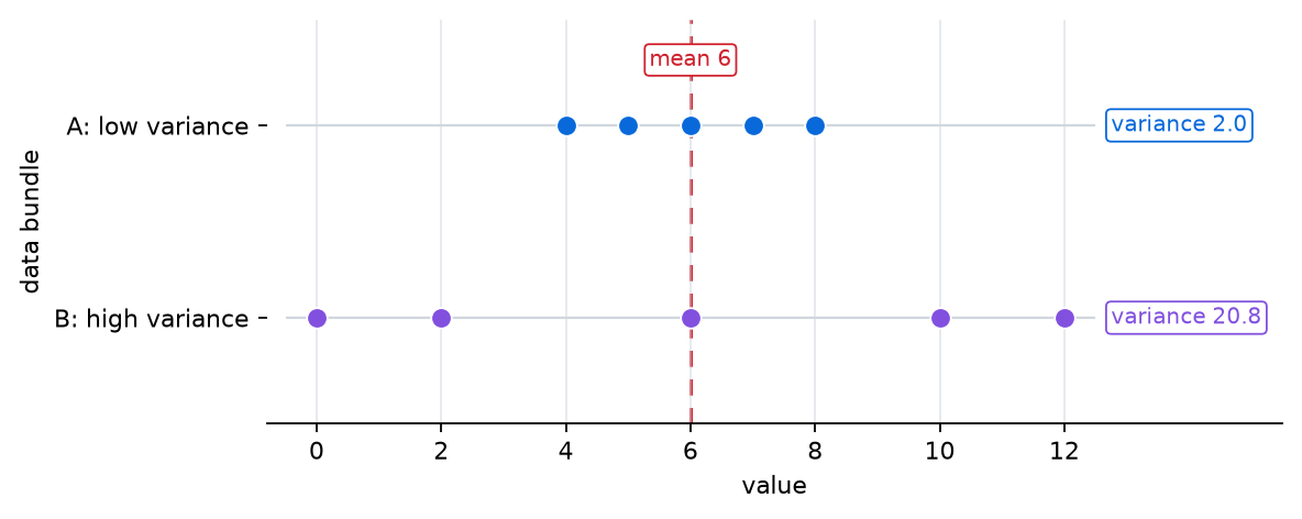
A: 4, 5, 6, 7, 8, B: 0, 2, 6, 10, 12
The mean of both bundles is 6.
But the two data bundles do not feel the same. In A, values gather near the mean. In B, values spread far away from the mean.
If we look only at the mean, the two data bundles may look similar. But in reality, stability, predictability, and risk may differ.
The chart below shows that even when the mean is the same, the spread can be different.
Distance from the Mean and Variance
Variance is the value that shows how widely values spread around the mean.
Squaring each value’s difference from the mean, then averaging those squares, summarizes the spread of the observed dataset.
The representative flow for calculating variance is the following.
- Compute the mean.
- Subtract the mean from each value.
- Square the difference.
- Take the mean of those squared values.
Writing the variance of this dataset itself as v gives:
This expression describes the spread of the given values, so it divides by their count, n. The sample variance commonly used to estimate population variance divides by n − 1 and serves a different purpose.
Values above the mean have positive differences, and those below it have negative differences. Adding the differences directly makes them cancel, while squaring gathers deviations from the mean as nonnegative values.
Calculating Variances of Two Datasets
The two datasets above, A: 4, 5, 6, 7, 8 and B: 0, 2, 6, 10, 12, both have mean 6.
| Calculation | A | B |
|---|---|---|
| Differences from the mean | −2, −1, 0, 1, 2 | −6, −4, 0, 4, 6 |
| Squared differences | 4, 1, 0, 1, 4 | 36, 16, 0, 16, 36 |
| Sum of squares | 10 | 104 |
| Variance: sum / 5 | 2 | 20.8 |
Although the means are equal, B's variance is 10.4 times A's. This quantifies the difference that B contains more values far from the mean.
Units of Variance and Standard Deviation
When learning variance, we also often meet standard deviation.
Standard deviation is the square root of the variance.
If data is measured in seconds, variance has units of seconds squared, while standard deviation has units of seconds. Taking the square root lets standard deviation compare spread in the original data’s units.
If A and B were response times in seconds, their standard deviations would be √2 ≈ 1.41 seconds and √20.8 ≈ 4.56 seconds. Even though both services have a mean response time of 6 seconds, B's response times are more widely spread.
Mean Loss and Differences Between Groups
In model evaluation, a mean can hide differences. Suppose 90 of 100 evaluation samples have loss 0.1, and the other 10 have loss 2.1. The mean loss is (90 × 0.1 + 10 × 2.1) / 100 = 0.3.
The overall mean is 0.3, but the last 10 samples have loss 2.1. If those 10 are images taken under the same conditions, we can check separately whether the model struggles under those conditions. This is why we inspect the loss distribution and group values alongside mean loss.
Checklist
- Can you explain distribution, mean, and variance as shape, center, and spread, respectively?
- Can you distinguish the distribution of observed data from a probability distribution?
- Can you calculate variances of 2 and 20.8 for the two datasets with mean 6?
- Can you distinguish the denominators used for a dataset’s own variance and for sample variance estimating population variance?
- Can you explain the relationship and units of variance and standard deviation?
- Can you explain how overall mean loss can hide large losses in a particular group?
Sources and References
- Barbara Illowsky, Susan Dean, Introductory Statistics, 2.2 Histograms, Frequency Polygons, and Time Series Graphs, OpenStax, checked 2026-07-20. Used to confirm that histograms help read the shape, center, and spread of large data bundles.
- Barbara Illowsky, Susan Dean, Introductory Statistics, 2.5 Measures of the Center of the Data, OpenStax, checked 2026-07-20. Used as support for explaining the mean as a representative measure of center.
- Barbara Illowsky, Susan Dean, Introductory Statistics, 2.7 Measures of the Spread of the Data, OpenStax, checked 2026-07-20. Used to confirm the explanation of variance and standard deviation as spread around the mean, squared deviations, and connection back to original units.