P2-5.4 Checking Probability and Statistics with Small Data¶

Section ID: P2-5.4 Version: v2026.09.15

Calculate the observed proportion of scores at least 60, then check the mean, median, and variance of eight scores. Change extreme values and compare means across samples to distinguish calculated values from estimates about a population.

Execution Environment¶

The code in this Section uses NumPy.

For the difference between notebook code cells and terminals, see Where to Run Commands. Run the code blocks in order from top to bottom.

If you use Google Colab, you can prepare NumPy in a code cell like this.

1
2

# This command installs NumPy inside a Colab/Jupyter code cell.
%pip install numpy

If you use a local PC, use the following command in your own terminal.

1

python -m pip install numpy

You can also inspect the full example code of this Section in the following file.

• p2_5_4_small_statistics.py

If you run it from the project root, you can use the following command.

1

python docs/assets/part-02/chapter-05/p2_5_4_small_statistics.py

Creating a Score Array¶

Start the calculation from a small data list.

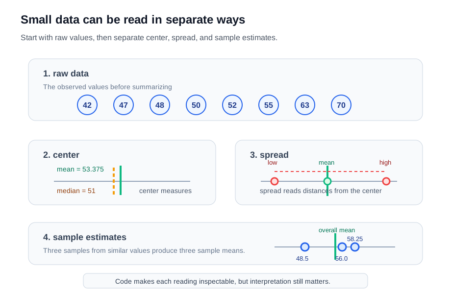
Put eight scores into the array data, and print the values and element count 8. This array is the input for the mean and variance calculations below.

 1
 2
 3
 4
 5
 6
 7
 8
 9
10

# This example imports NumPy to prepare mean, median, and variance calculations for small data.
import numpy as np

# data is the small score dataset used to check mean, median, and variance.
data = np.array([42, 55, 48, 63, 52, 50, 47, 70])

print(data)

# size shows how many values the dataset contains.
print(data.size)

You can read the output like this.

1
2

[42 55 48 63 52 50 47 70]
8

Here, data is not the whole of reality. It is the small bundle of data we observed. In the language of the previous Section, it can be read like a sample.

At this stage, the important questions are what these numbers record, how they were collected, and whether they can be seen as representative of the whole.

Code can perform the calculation, but a person has to decide what the data means.

Proportion of Scores at Least 60¶

data >= 60 checks whether each score is at least 60. True means the condition is met; False means it is not. Counting the true elements with np.count_nonzero gives 2, corresponding to the scores 63 and 70.

1
2
3
4
5
6

at_least_60 = data >= 60
count_at_least_60 = np.count_nonzero(at_least_60)
observed_ratio = count_at_least_60 / data.size
print(at_least_60)
print(count_at_least_60)
print(observed_ratio)

1
2
3

[False False False  True False False False  True]
2
0.25

Of the eight observed scores, 2 / 8 = 0.25, or 25%, are at least 60. If one of these eight scores is selected with equal probability, the probability of a score of at least 60 is exactly 0.25. For a larger population, this proportion is an estimate of that probability; the collection method and sample representativeness must also be checked.

Calculating the Mean¶

The mean summarizes the center of the data into one number.

Applying np.mean to data gives the mean 53.375.

1
2
3

# mean_value is the mean that summarizes all values in data as one center value.
mean_value = np.mean(data)
print(mean_value)

The output is 53.375.

This number stands in for the following calculation.

The mean is convenient, but one mean alone cannot tell you the full shape of the data. The mean shows the center, but how widely the values are spread must be checked separately.

Also, the mean can be shaken by one extremely large or small value. One representative value you can look at together in that situation is the median.

Extreme Values and the Median¶

The median is the middle value after sorting values in order. With an even number of values, use the mean of the two middle values.

Sorting the original eight scores places 50 and 52 in the middle. Their average, (50 + 52) / 2 = 51, is the median shown in the opening diagram.

1
2

print(np.sort(data))
print(np.median(data))

1
2

[42 47 48 50 52 55 63 70]
51.0

In the next data, one value is unusually large.

Include the large value 100 in skewed_data and compare the mean and median. The expected results are 30.0 and 13.0, respectively.

1
2
3
4
5

# skewed_data includes the extreme value 100 to compare how mean and median react.
skewed_data = np.array([10, 12, 13, 15, 100])

print(np.mean(skewed_data))
print(np.median(skewed_data))

The output is 30.0, 13.0.

The mean becomes 30.0 because it is strongly affected by 100. But the median is 13.0, the middle of the sorted values.

Because the mean calculates the center by adding all values, it can be shaken by one extremely large or small value. The median, by contrast, looks at the middle position after sorting, so it is relatively less shaken by an outlier.

In real data, long one-sided distributions appear often. In data like user usage time, waiting time, response latency, or income, where some values can become very large, looking only at the mean can misread what the data typically looks like.

Deviations, Squared Deviations, and Variance¶

Variance is the number that looks at how widely values are spread around the mean.

First, subtract the mean from each value.

Print the deviations obtained by subtracting the mean from data, rounded to three decimal places. They show how far each value is above or below the center.

1
2
3

# centered shows how far each value is from the mean.
centered = data - np.mean(data)
print(np.round(centered, 3))

You can read the output like this.

1

[-11.375   1.625  -5.375   9.625  -1.375  -3.375  -6.375  16.625]

These values show how far each datum is from the mean. For example, 42 is 11.375 below the mean, 70 is 16.625 above the mean, and 55 is 1.625 above the mean.

Next, square those distances.

Square the deviation array centered. Squared deviations prevent negative and positive differences from canceling each other.

1
2
3

# squared_deviations squares the deviations so both negative and positive gaps count as spread.
squared_deviations = centered ** 2
print(np.round(squared_deviations, 3))

You can read the output like this.

1

[129.391   2.641  28.891  92.641   1.891  11.391  40.641 276.391]

Variance can then be seen as the value obtained by averaging these squared gaps.

Calculating the mean of squared deviations with np.var(data) gives the variance 72.984375.

1
2

# np.var(data) summarizes the spread of data as one variance value.
print(np.var(data))

The output is 72.984375.

Variance Denominators and ddof¶

np.var(data) divides the sum of squared deviations of the observed values by their count, N. Even when data comes from a sample, this calculation can describe the spread of that dataset itself.

The sample variance commonly used to estimate population variance divides the same sum by N − 1. In NumPy, specify ddof=1. For independent samples drawn from the same distribution, this correction reduces the downward bias in variance estimation caused by using the sample mean to calculate squared deviations.

1
2

print(np.var(data))
print(np.var(data, ddof=1))

1
2

72.984375
83.41071428571429

Both calculations use the same data and the same sum of squared deviations, 583.875. The first value is 583.875 / 8; the second is 583.875 / 7. The data has not changed: the denominator was chosen for a different calculation purpose.

The denominator in np.var is N − ddof. Setting ddof=1 does not fix missing or overrepresented groups. Correcting the denominator and checking the sample collection method are separate tasks.

Comparing Sample Means¶

Treat the 12 values in population_like as a small population. Compare the means of the three selected samples in samples with the population mean 54.75.

 1
 2
 3
 4
 5
 6
 7
 8
 9
10
11
12
13
14
15

# The 12 values in population_like are the small population in this example.
population_like = np.array([42, 45, 47, 48, 50, 52, 55, 58, 61, 63, 66, 70])

# samples are smaller groups used as if we observed only part of population_like.
samples = np.array([
    [42, 47, 50, 55],
    [48, 52, 63, 70],
    [45, 55, 58, 66],
])

print(np.mean(population_like))

# Check each sample in order to see whether its mean changes.
for sample in samples:
    print(sample, np.mean(sample))

You can read the output like this.

1
2
3
4

54.75
[42 47 50 55] 48.5
[48 52 63 70] 58.25
[45 55 58 66] 56.0

The population mean in this example is 54.75. Depending on the selected sample, the sample means are 48.5, 58.25, and 56.0.

The three samples were selected by hand for comparison, not drawn at random. There is one population mean, but sample means can vary with the sample, so a sample mean is an estimate of the population mean.

Calculated Results and Sample Representativeness¶

Code calculates mean and variance quickly. But how to interpret the numbers is a separate issue.

For example, if the mean is 53.375, it is risky to jump straight to conclusions like "the average of all users of this service is 53.375," "this data perfectly represents the whole," or "the variance is large, so the data is bad."

A more careful wording is closer to "the mean in this data bundle is 53.375," "the values are spread to some degree around the mean," and "whether this data represents the whole must be checked together with the collection method and sample composition."

The same attitude is needed in AI data. The mean of training data is a summary value calculated inside the training dataset, the score on test data is an evaluation value obtained from the test sample, and real-world performance is something that must be checked through separate samples, post-deployment observation, and continued evaluation.

Comparing Different Extreme Values¶

Change the last value in skewed_data from 100 to 1000 and print the mean and median again. The mean increases to (10 + 12 + 13 + 15 + 1000) / 5 = 210, while the median stays at 13.

Now change the last value to 14. The sorted values are 10, 12, 13, 14, 15, with mean 12.8 and median 13. Compare the two outputs to see how much one large value raised the mean.

Copy the array with copy() to preserve the original, then change only its last element, [-1]. Each output row lists the changed value, mean, and median.

1
2
3
4

for last_value in [1000, 14]:
    changed_data = skewed_data.copy()
    changed_data[-1] = last_value
    print(last_value, np.mean(changed_data), np.median(changed_data))

1
2

1000 210.0 13.0
14 12.8 13.0

Checklist¶

• You can distinguish an observed proportion from an estimate of a population probability.
• You can make a small data list as a NumPy array.
• You can calculate the mean with np.mean.
• You can calculate the median with np.median.
• You can explain that the mean can be shaken by an outlier.
• You can check how far each value is from the mean.
• You can calculate the variance with np.var.
• You can explain that ddof=1 can be used in sample-variance calculation.
• You can explain that the sample mean can change when the sample changes.
• You can separate code output from issues of data collection method, sample representativeness, and interpretation.
• You can connect the definitions of mean, median, and variance to actual numbers and code output.

Sources and References¶

• NumPy Developers, numpy.array, NumPy Reference, checked 2026-07-20. Used to confirm the example that creates a NumPy array from a small numeric list.
• NumPy Developers, numpy.ndarray.size, NumPy Reference, checked 2026-07-20. Used to confirm the data.size example for reading the number of array elements.
• NumPy Developers, numpy.mean, NumPy Reference, checked 2026-07-20. Used to confirm arithmetic mean and array-mean calculations.
• NumPy Developers, numpy.median, NumPy Reference, checked 2026-07-20. Used to confirm that the median is the middle value of a sorted copy, or the average of the two middle values for an even number of values.
• NumPy Developers, numpy.var, NumPy Reference, checked 2026-07-20. Used to confirm variance, ddof, and the difference between population-variance and sample-variance calculation settings.

• Barbara Illowsky, Susan Dean, Introductory Statistics, 1.2 Data, Sampling, and Variation in Data and Sampling, OpenStax, checked 2026-07-20. Used to confirm the statistical background that samples should represent the population and that sampling methods can introduce variation.

• NumPy Developers, numpy.count_nonzero, NumPy Reference, checked 2026-09-15. Used to verify counting elements that satisfy a condition in a Boolean array.