P2-6.3 The Intuition of Gradient Descent
Section ID:
P2-6.3Version:v2026.09.15
Gradient descent calculates the objective function’s gradient at the current parameters and changes the parameters in the opposite direction. The learning rate multiplies the gradient to control the amount of movement.
Current Loss of the Line Model
We use data for predicting scores from study time.
| Student | Study time x | Actual score y |
|---|---|---|
| A | 1 | 55 |
| B | 2 | 65 |
| C | 3 | 80 |
| D | 4 | 90 |
For the current line \(\hat{y} = 8x + 45\), the predictions are 53, 61, 69, 77, below the actual scores by 2, 4, 11, 13. The mean squared error is (4 + 16 + 121 + 169) / 4 = 77.5.
The objective is to reduce this loss by changing slope a and intercept b.
The movement can be represented as a learning loop:
flowchart TD
  P["Current parameters a, b"]
  L["Predictions and MSE<br/>for all four students"]
  G["Both partial derivatives<br/>at the same current position"]
  U["[a, b] − η × gradient"]
  P --> L --> G --> U --> P
The Slope at the Current Position
Gradient descent is often compared to descending a mountain: inspect the nearby slope and take small steps downhill.
The current position represents the model parameters, height represents loss, and downhill represents the direction in which loss decreases.
The analogy has limits. In actual model training, we do not see the entire map at once. We read the direction near the current position, move a little, and check again.
Gradient descent is therefore an iterative method that seeks gradual improvement using current information, rather than jumping directly to the answer.
In the study-time example, if the current line underpredicts students C and D, we repeatedly check whether slightly increasing a or adjusting b reduces loss instead of guessing a perfect line at once.
Opposite to the Gradient
The gradient is associated with the direction of the fastest local increase in the function value. For a loss function, it points toward increasing loss.
AI training usually seeks to reduce loss, so it moves opposite to the gradient. The gradient points toward increasing loss, and the opposite direction points toward decreasing loss.
This is the meaning of descent: we calculate a gradient in order to go down.
For a differentiable objective with a nonzero gradient, a sufficiently small step opposite to the gradient reduces the objective value. A large step in that same direction can increase loss.
Learning Rate and Movement Size
Knowing a direction of decreasing loss does not justify a large jump. The current gradient describes the local neighborhood. Too large a step may overshoot a lower point.
The learning rate controls how much to move. Too small a rate produces slow progress; an appropriate rate can steadily reduce loss; too large a rate can overshoot a good position or make loss fluctuate.
The actual movement is the learning rate multiplied by the gradient. Even at the same learning rate, movement distance changes when gradient magnitude changes.
For example, increasing a too much at once might reduce student D’s error while overshooting for students A and B. Too small a change makes improvement slow even when the direction reduces loss. The learning rate controls this step size.
The Gradient Descent Update
Gradient descent is commonly written as:
The symbols denote the following values.
| Symbol | Introductory meaning |
|---|---|
| \(\theta\) | Parameters adjusted by the model |
| \(J(\theta)\) | The objective function to reduce |
| \(\nabla J(\theta)\) | Direction of increasing loss at the current position |
| \(\eta\) | Learning rate, a movement coefficient multiplying the gradient |
| \(-\eta \nabla J(\theta)\) | A small movement toward decreasing loss |
Here, \(\theta\) is [a, b], and \(J\) is the mean squared error across the four students. The formula compresses the calculation current parameters − learning rate × gradient.
One Update of Slope and Intercept
Writing each student’s predicted − actual value as \(r_i\), the current errors are −2, −4, −11, −13. Differentiating MSE with respect to each parameter gives:
Changing a affects predictions more for students with greater study time x, so the first expression multiplies by x_i. Changing b shifts every prediction by the same amount.
At learning rate 0.01, the update is:
a_new = 8 − 0.01 × (−47.5) = 8.475b_new = 45 − 0.01 × (−15) = 45.15
Predicting with the new line reduces MSE from 77.5 to about 54.76. For the next update, recalculate the gradient at [8.475, 45.15].
Recalculating at the New Position
The first update uses the gradient calculated at the same pre-update position [8, 45] for both parameters. This differs from changing only a first and using that changed value to calculate the gradient for b.
At the new position [8.475, 45.15], predictions are 53.625, 62.1, 70.575, 79.05. The errors, predicted minus actual, are now −1.375, −2.9, −9.425, −10.95, so the gradient must be recalculated.
| Pre-update position [a, b] | Gradient at that position | Position after update with η=0.01 | MSE after update |
|---|---|---|---|
| [8, 45] | [−47.5, −15] | [8.475, 45.15] | About 54.7584 |
| [8.475, 45.15] | [−39.625, −12.325] | [8.87125, 45.27325] | About 38.9750 |
The second update gives a=8.475−0.01×(−39.625)=8.87125 and b=45.15−0.01×(−12.325)=45.27325. Even with the same learning rate, the movement changes because the gradient changes. This is full-batch gradient descent: every update uses the loss over all four students to calculate the gradient.
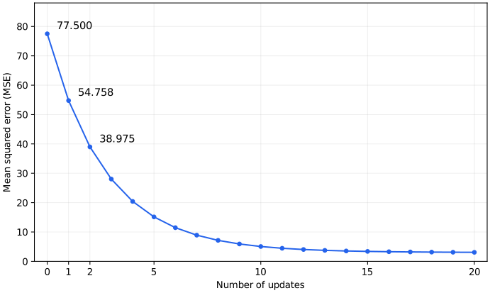
The horizontal axis counts updates, and the vertical axis shows MSE at each step. Using the same four students, the run starts at [8, 45] with learning rate 0.01 and recalculates the gradient every time. Step 0 is the loss before any update. This graph records loss over 20 updates; it is not a landscape in parameter space.
Comparing Loss Across Learning Rates
Starting from [8, 45] with gradient [-47.5, -15], change only the learning rate and take one step.
| Learning rate | New a | New b | MSE after the step |
|---|---|---|---|
| 0.001 | 8.0475 | 45.015 | About 75.04 |
| 0.01 | 8.475 | 45.15 | About 54.76 |
| 0.2 | 17.5 | 48 | About 409.63 |
All three steps move opposite to the gradient, but a learning rate of 0.2 greatly increases loss. At 0.001, the decrease is small. Both the direction and the amount of movement need to be chosen appropriately.
Conditions Affecting Convergence
Gradient descent is powerful, but it does not automatically guarantee a perfect answer.
Several conditions affect the result.
| Condition | Why it matters |
|---|---|
| Initialization | The path may depend on the starting position. |
| Learning rate | Too small can be slow; too large can be unstable. |
| Loss landscape | There may be valleys, flat regions, and multiple low points. |
| Data | Loss is calculated from data and is affected by its quality. |
| Iterations | Too few may leave the model undertrained; too many may lead to overfitting. |
Gradient descent moves toward improvement under given criteria and conditions. It does not automatically resolve every real-world condition.
Convergence and Stopping Training
Convergence means that changes in parameters or the objective become small as iterations approach a limiting value. An implementation can set a maximum iteration count and check whether the change in loss between consecutive updates or the gradient magnitude falls below a chosen tolerance. A small change in loss alone does not establish arrival at an optimum: an excessively small learning rate may simply prevent meaningful movement.
Early stopping can instead use performance on validation data. For example, training can stop when validation loss has not improved for a specified period, even while training loss decreases. Convergence of the objective and performance on new data are separate judgments. Test data is not used to repeatedly choose the stopping point.
What Happens If the Old Gradient Is Reused?
After the first update, start at [8.475, 45.15] and reuse the original [-47.5, -15] instead of recalculating the gradient. What are the next parameters with learning rate 0.01? Compare them with the second update in the table.
Answer: The result is a=8.95, b=45.3, different from [8.87125, 45.27325] obtained by recalculating at the current position. In this example, reusing the old gradient also reduces MSE, to about 36.1588. A larger decrease in one step, however, does not guarantee that the direction and magnitude will remain appropriate for subsequent updates. Basic gradient descent uses the gradient at the current position.
Checklist
- You can explain gradient descent as repeated movement to reduce loss.
- You can connect the gradient to increasing loss at the current position.
- You can explain why reducing loss requires moving opposite to the gradient.
- You can explain the learning rate in terms of movement size.
- You can read the update as taking a small step opposite to the gradient from the current values.
- You can explain the influence of initialization, learning rate, loss landscape, data, and iteration count.
- You can connect reducing loss to actual changes in parameters.
- You can distinguish the gradient direction from the opposite direction used for descent.
Sources and References
- Ian Goodfellow, Yoshua Bengio, Aaron Courville, Deep Learning, Chapter 8: Optimization for Training Deep Models, MIT Press, 2016, checked 2026-09-15. Used to support the deep-learning optimization context of cost functions, parameters, gradient-based movement, gradient descent, and learning rate.
- Stephen Boyd, Lieven Vandenberghe, Convex Optimization, Cambridge University Press, 2004, checked 2026-07-20. Used as supplementary support for optimization problems and gradient-based repeated movement in the mathematical optimization context.