P2-15.1 A Small Procedure for Translating Formulas into Code¶

Section ID: P2-15.1 Version: v2026.07.23

In Part 2, we looked at formulas, Python, NumPy, Pandas, and Matplotlib separately. Now we bind that flow into one procedure. The goal is not to prove difficult formulas, but to have a procedure for translating a simple formula into code and checking the result.

When you study machine learning, formulas such as the loss function, mean, variance, and linear combination keep appearing. To avoid freezing as soon as you see a formula, you need the habit of turning symbols into a computation procedure.

A Place to Tie Together Concepts from Earlier Chapters Again¶

This section is the place where concepts learned separately in Part 2 are tied together again through one example. Rather than adding a large new theory, it shows what should be checked when the representative concepts from earlier chapters actually move together.

So the core of this section is not memorizing a new formula, but connecting tools you already saw to one problem through a procedure.

Core Criteria: A Small Procedure for Translating Formulas into Code¶

• You can first distinguish the variables and the data bundle in a formula.
• You can translate sigma summation into a Python loop or a NumPy computation.
• You can compute mean squared error with a small code example.
• You can explain the flow of checking the code result with numbers, a table, and a plot.
• You can obtain a minimum procedure for reading machine-learning formulas in Part 3.

The First Connections to Hold in This Section¶

• Turn the symbols of the formula into code variables.
• First look at the repeated computation per sample.
• Read the same computation again as a NumPy array expression.
• Check the final number, the intermediate values, and the plot together.

Three Criteria¶

The Basic Order for Translating a Formula into Code¶

When turning a formula into code, do not write code immediately. Read it in the following order first.

flowchart TD
  A["1. formula<br/>read the formula"]
  B["2. symbols<br/>decide what the symbols mean"]
  C["3. data shape<br/>distinguish scalar, vector, table"]
  D["4. computation<br/>translate to loop or array math"]
  E["5. check<br/>verify with small numbers"]

  A --> B --> C --> D --> E

The key point is not to convert the formula into code all at once. First decide what the symbols point to, then check whether the values are single values or bundles, and only then compute.

Read Mean Squared Error as an Example¶

Mean squared error (MSE) is the value obtained by squaring the difference between the predicted values and the actual values and then averaging those squares.

At first sight it may look complex, but if you split the symbols, it becomes the following.

This formula can be read as: "compute the error of each sample, square it, add them all, and divide by the count."

First Translate It into a Small Python Loop¶

Here, rather than shortening it immediately with NumPy, we first check the computation flow with a loop.

Problem situation:

• even if you read the formula, you may not immediately connect each symbol to a loop and variable in code

Input:

• a list of actual values, actual
• a list of predicted values, predicted

Expected output:

• a list of squared errors by sample
• the mean squared error value

Concept to check:

• sigma summation can be translated into a loop or an array computation
• when translating a formula into code, it is safer to separate per-sample computation from the final averaging step
• the loop version reveals the meaning of the computation before the condensed NumPy expression

 1
 2
 3
 4
 5
 6
 7
 8
 9
10
11
12

# This example computes errors between actual and predicted values and translates a loss formula into code.
actual = [3.0, 5.0, 7.0]
predicted = [2.5, 5.5, 8.0]

squared_errors = []

for y, y_hat in zip(actual, predicted):
    error = y - y_hat
    squared_errors.append(error ** 2)

mse = sum(squared_errors) / len(squared_errors)
print(mse)

This code follows almost each part of the formula directly.

This step is short and simple, but important. It lets you check by hand what computation procedure the formula represents.

Then Shorten the Same Computation with NumPy¶

After understanding the computation flow, you can write it more briefly with a NumPy array.

Problem situation:

• after understanding the meaning through a loop, you should be able to express the same formula again as a shorter array computation

Input:

• the array of actual values, actual
• the array of predicted values, predicted

Expected output:

• the error array, errors
• the squared error array, squared_errors
• the mean squared error, mse

Concept to check:

• NumPy array operations reduce sigma computation into a vectorized expression
• even in shorter code, the computation steps keep the same meaning as in the loop version

 1
 2
 3
 4
 5
 6
 7
 8
 9
10
11

# This example computes errors between actual and predicted values and translates a loss formula into code.
import numpy as np

actual = np.array([3.0, 5.0, 7.0])
predicted = np.array([2.5, 5.5, 8.0])

errors = actual - predicted
squared_errors = errors ** 2
mse = np.mean(squared_errors)

print(mse)

In NumPy, subtracting one array from another computes values at matching positions. This connects directly to vectorization from Part 2 Chapter 11.

Still, shorter NumPy code does not always mean easier understanding from the start. In this section, the formula and code are connected in the order confirm the meaning with a loop, then shorten the expression with NumPy.

Do Not Look Only at One Final Number¶

MSE eventually becomes a single number. But when checking the computation process, it is better to look at intermediate values together.

Problem situation:

• if you look only at the final MSE value, it is hard to read immediately in which sample the error became larger

Input:

• errors computed above
• squared_errors
• mse

Output:

• the intermediate error array and the final mean squared error value

Concept to check:

• printing intermediate values together lets you check what number each stage of the formula actually produces
• you can compare directly the sign of the error and the value after squaring

1
2
3
4

# This example computes errors between actual and predicted values and translates a loss formula into code.
print(errors)
print(squared_errors)
print(mse)

If the output looks similar to the following, you can confirm the meaning of each stage.

1
2
3

[ 0.5 -0.5 -1. ]
[0.25 0.25 1.  ]
0.5

An error has a direction. The sign changes depending on whether the prediction was smaller or larger than the actual value. But squared error never becomes negative. That is why MSE becomes a metric that looks at the size of the error on average.

You Can Also Check It with a Plot¶

If you look only at numbers, it may not be obvious at once in which sample the error is large. If you draw the actual and predicted values side by side with Matplotlib, it becomes easier to see where the error grows.

Problem situation:

• numerical output alone may make it hard to grasp at a glance where and how large the sample-by-sample differences are

Input:

• the actual-value array, actual
• the predicted-value array, predicted
• the sample index, index

Output:

• a line plot comparing actual and predicted values

Concept to check:

• a plot does not replace loss calculation, but becomes a supporting tool for interpreting the error distribution
• even with the same numeric result, visualization helps you read more quickly in which interval the difference was large

 1
 2
 3
 4
 5
 6
 7
 8
 9
10
11
12
13

# This example computes errors between actual and predicted values and translates a loss formula into code.
import matplotlib.pyplot as plt

index = np.arange(len(actual))

fig, ax = plt.subplots()
ax.plot(index, actual, marker="o", label="actual")
ax.plot(index, predicted, marker="o", label="predicted")
ax.set_xlabel("sample index")
ax.set_ylabel("value")
ax.set_title("Actual and predicted values")
ax.legend()
plt.show()

The output image shows the gap between actual and predicted values for each sample.

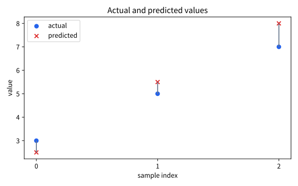
The loop calculation, NumPy calculation, and plot-saving flow in this section can be rerun together with p2_15_1_formula_to_code_mse.py. This script prints loop mse, errors, squared errors, and numpy mse, and saves actual-predicted-mse.png in the same asset folder.

This plot does not calculate MSE instead of you. It helps you inspect with your eyes the difference before it is compressed into one number.

Case Study¶

Case 1. Why You Cannot Write Code Immediately After Seeing a Loss Formula¶

Suppose a learner sees the mean squared error formula for the first time and gets stuck at the question, "How do I translate this into Python?" A person may be able to read the shape of the formula, yet fail to connect immediately which value is one number, which value is a bundle of samples, and into what repetition sigma turns in code.

If you jump immediately into a one-line NumPy expression at that point, you may obtain the result but miss the procedure. If you first keep actual and predicted as small lists, then compute each sample's error, square it, add everything, and divide by the count with a loop, the structure of the formula changes into a computation procedure.

Then, by shortening the same calculation with a NumPy array, you can read the condensed expression separately from the meaning of the calculation. In other words, the loop is the foothold for interpreting the formula, and NumPy is the expression that writes that calculation more concisely.

This case continues directly into formula reading after Part 3. What matters first is not writing code quickly. It is having the sense of changing symbols into a procedure of input, repetition, and output.

Checklist¶

• Can you explain what \(y_i\), \(\hat{y}_i\), \(n\), and \(\sum\) mean in the MSE formula?
• Can you write the same calculation both as a Python loop and as a NumPy array computation?
• Can you explain the difference among errors, squared_errors, and mse?
• Can you explain why intermediate values should be checked instead of looking only at the final result?
• Can you explain that a plot helps interpretation instead of replacing the computation?
• Can you first separate symbols, data shape, and computation procedure when translating a formula into code?

Sources and References¶

• Python Software Foundation, An Informal Introduction to Python, Python documentation, checked on 2026-07-20. https://docs.python.org/3/tutorial/introduction.html Used as the basis for the numeric, list, and basic calculation expressions in the formula-to-code example.
• NumPy Developers, NumPy: the absolute basics for beginners, NumPy documentation, checked on 2026-07-20. https://numpy.org/doc/stable/user/absolute_beginners.html Used as the basis for array creation, array operations, and vectorized calculation with np.mean.
• Matplotlib Developers, Quick start guide, Matplotlib documentation, checked on 2026-07-20. https://matplotlib.org/stable/users/explain/quick_start.html Used as the basis for checking calculation results with Figure, Axes, plot, labels, and legends.