P3-1.1 What Is Data Modeling Trying to Achieve
Section ID:
P3-1.1Version:v2026.09.19
As soon as the reader enters Part 3, they meet words such as sample, feature, baseline, output structure, and target. These terms do not stand alone. The outer judgment that decides what counts as one case, which values remain, what gets compared, and in what result format the process closes is data modeling.
If data modeling is understood only as organizing storage structures, it can sound like making existing tables look tidier. In Part 3, this book uses the term more broadly to mean designing samples and representations for a question. This is the scope chosen for the book, not a standard definition that replaces data modeling in databases. The task is to decide which questions the available source data should enable us to answer.
The most common early confusion is to treat how should we store the database? and how should we build a problem structure that AI can read? as if they were the same task. They are connected, but their goals differ.
| Point of comparison | A view centered on storage structure | The data-modeling view of Part 3 |
|---|---|---|
| First question | How should records be stored and retrieved without loss? | How should samples and comparison structure be built so a question can be answered? |
| Representative unit | one log row, one event, one sensor reading | one action, one recent segment, one entity as an analysis sample |
| Main concern | Is it stored without omission, linked correctly, and traceable? | What can be compared, and which features should remain? |
| Immediate result | raw log tables, event tables, joinable storage structure | summary tables, feature tables, baseline comparison tables, output structures for review |
| Question in this Part | It may still be a starting point, but it is not the end point | The central question handled throughout Part 3 |
If storage structure is the frame for not losing records, data modeling is closer to the frame for building comparison structure that can answer a question. Check whether the stored data already has the sample unit and information required by the question, and change its representation when necessary. Raw records are also a dataset; not every analysis requires a new summary table.
Suppose there is a record of automatically executed actions. The source data may contain time-step sensor values, control parameters, and start and end times for each action. That structure may be sufficient for storage and traceability. But in that state, it is still difficult to answer questions such as was this action different from the usual ones?, is repeatability unstable in the recent segment?, or what should a person review first?
What data modeling is trying to achieve here is simple. It makes the connection between questions and records explicit so that people can compare them and models can use them. In this action-comparison example, we make four decisions.
- Decide what should count as one sample.
- Build features that describe that sample.
- Set a baseline for what the recent state will be compared against.
- Decide the output structure, such as whether the final result is for human review or a candidate prediction target.
These are design questions for this example, not four mandatory column types for every dataset. Raw time series, images, or documents can be inputs, and some tasks do not compare against a historical baseline.
At this point, the relation between data modeling and data science also needs to be fixed. Data science is the broader flow that includes data collection, cleaning, exploration, summarization, comparison, interpretation, prediction, and connection to decision making. Inside that larger flow, the data modeling that Part 3 focuses on is closer to the front-end judgment that turns source data into a problem structure for AI learning and analysis. In other words, Part 3 is not the Part that teaches all of data science. It teaches data handling needed to understand AI by connecting questions, representations, and interpretation.
To see this more clearly, place the outputs data modeling is actually trying to create side by side.
| What it tries to achieve | Why it is needed | Question that it connects to later |
|---|---|---|
| Sample unit | Because we must decide what counts as one case | What does one row mean? |
| Feature table | Because descriptive values for comparison and learning must be built | Which values should remain? |
| Baseline comparison structure | Because the recent state must be read against the usual state | What should it be compared to? |
| Output structure | Because human review and prediction targets must not be mixed | What should the result be emitted as? |
The important point in this table is that data modeling is not yet the model selection stage. At this stage, before classifier names or deep-learning structures, we first have to decide what table gets built and what comparison becomes possible. Only then do X, y, evaluation, and baseline models stop floating in midair in the later machine-learning Parts.
The diagram shows the flow chosen for this action-comparison example. It is not a mandatory procedure for all data.
flowchart TD
  A["Raw time-series logs"] --> B["Choose one sample unit"]
  B --> C["Summarize into features"]
  C --> D["Compare with a baseline"]
  D --> E["Decide output structure"]
  E --> F["Review candidate or prediction-ready table"]
Level, spread, and direction ask different questions about an action
The following fictional records are used for explanation. action_id identifies an action, t_sec is time since its start in seconds, flow_rate is flow in L/min, and pressure is pressure in kPa. A value of 1 in valve_open means the valve is open. Assume one measurement at 0, 1, and 2 seconds for each action.
| action_id | t_sec | flow_rate | pressure | valve_open |
|---|---|---|---|---|
| A-101 | 0.0 | 24.8 | 101.2 | 1 |
| A-101 | 1.0 | 25.1 | 101.0 | 1 |
| A-101 | 2.0 | 23.9 | 102.4 | 1 |
| A-102 | 0.0 | 24.7 | 100.9 | 1 |
| A-102 | 1.0 | 24.8 | 101.1 | 1 |
| A-102 | 2.0 | 24.8 | 101.0 | 1 |
Flow in A-101 rises slightly and then falls at the end. The three values in A-102 are close together, and its final two values are equal. To compare this difference, we group one action as one sample. The six rows are measurements from two actions, not six actions.
To describe numerically how the actions differ, first separate the questions. Overall flow level, spread among measurements, and a decline at the end are different properties. The numbers we retain depend on which question we ask.
Mean: what is the overall level of the measurements?
The mean is the sum of the values divided by their count. Here, flow_mean contains the mean of the three flow measurements in each action.
- A-101:
(24.8 + 25.1 + 23.9) / 3 = 24.60 L/min - A-102:
(24.7 + 24.8 + 24.8) / 3 ≈ 24.77 L/min
A-101 has a slightly lower mean flow. The mean alone does not tell us when flow fell. For example, 23, 24, 25 and 25, 24, 23 both have a mean of 24, but one rises and the other falls. Summarizing the level loses the time order.
The chart uses identical axes for both actions. Dots are observations, dashed lines are means, and thick segments mark the final observed interval. Connecting lines help read the order of measurements; they do not establish the actual path between observations.
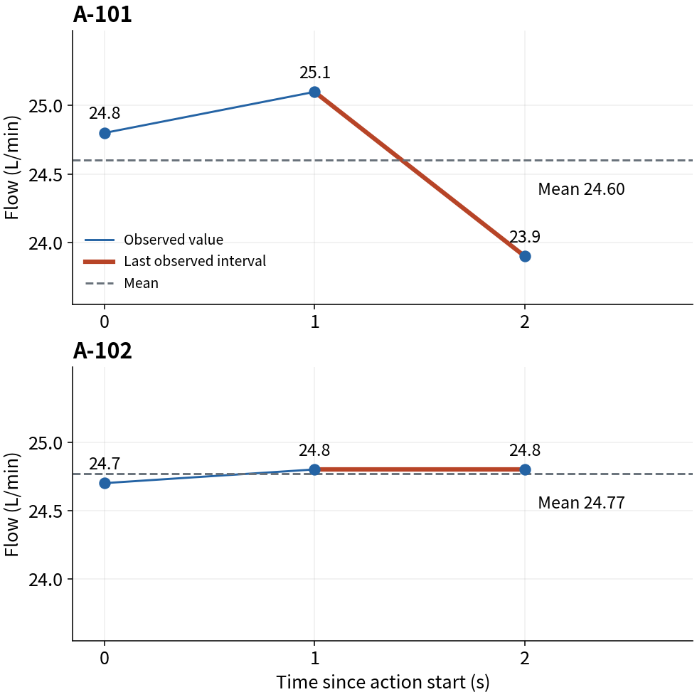
A-101 spreads farther around its mean and falls in the final interval. A-102 stays close to its mean. The horizontal mean lines alone cannot convey these shapes. We will distinguish spread from direction below.
Pressure is averaged in the same way and stored in pressure_mean. For A-101, (101.2 + 101.0 + 102.4) / 3 ≈ 101.53 kPa; for A-102, the result is 101.00 kPa. This lets us compare the overall pressure level alongside changes in flow; it is not itself a fault diagnosis.
Standard deviation: how far are the values spread around the mean?
Standard deviation describes the spread of values around their mean. It is zero when all three values are equal and increases as the values spread farther from the mean. It does not indicate whether they rise or fall over time.
Here, flow_std uses the sample standard deviation formula. Start by finding the differences from A-101's mean of 24.6.
- The differences are
24.8−24.6 = 0.2,25.1−24.6 = 0.5, and23.9−24.6 = −0.7. - Positive and negative differences cancel if added directly, so square each one. Their squared sum is
0.2² + 0.5² + (−0.7)² = 0.78. - For sample standard deviation, divide this sum by
number of values−1: here,0.78 / (3−1) = 0.39. - Take the square root to undo the squaring:
√0.39 ≈ 0.62 L/min. Standard deviation has the same unit as the original flow measurements.
This calculation convention is used when estimating a larger population's spread from a sample, hence the denominator 2 rather than 3. Here we use it to summarize three measurements; we do not infer the condition of all equipment from two actions. Applying the same calculation to A-102 using the unrounded mean gives approximately 0.06 L/min. In these records, A-101's flow values are therefore more widely spread around their mean.
The sequences 23, 24, 25 and 25, 24, 23 also have the same sample standard deviation: 1. Reversing their order leaves their distances from the mean unchanged. A large standard deviation and a steep final decline are different statements.
Final-interval slope: in which direction and how quickly did flow change?
To examine a decline at the end, use the change in value divided by elapsed time, or slope. Here the final interval runs from 1 to 2 seconds, and its slope is stored in late_drop_rate. Despite drop in the name, the sign is retained, so a rise can produce a positive value.
- A-101:
(23.9−25.1) / (2−1) = −1.2 L/min/s - A-102:
(24.8−24.8) / (2−1) = 0.0 L/min/s
L/min/s describes how much flow, measured in L/min, changes per second. Negative means decline, positive means rise, and zero means the two endpoint values are equal. Over the same time interval, −1.2 is a steeper decline than −0.2. This does not establish that flow changed at a constant rate between the two observations.
Baseline difference: how does the interval compare with its usual behavior?
Observing a decline does not establish that it differs from usual behavior. In this fictional example, assume a separately established usual final-interval slope of 0.0 L/min/s under the same conditions. This is the comparison baseline; it was not estimated from the six rows above.
Calculate baseline_gap as current action slope−baseline slope. A-101 gives −1.2−0.0 = −1.2 L/min/s, and A-102 gives 0.0−0.0 = 0.0 L/min/s. A negative difference means the current slope is lower than the baseline. If the baseline were −1.0, A-101's difference would be −0.2. Thus, the current slope and the baseline difference are different concepts.
Next, define an illustrative rule for selecting actions for human review: assign review if baseline_gap < −0.5 L/min/s, and no_flag otherwise. Exactly −0.5 receives no_flag. This threshold is an assumed rule connecting a metric to review, not a fault criterion validated on real equipment.
Combining values chosen for different questions into one action row
Combining the calculated values gives the following summary table. Means and standard deviations are displayed to two decimal places; calculations use unrounded values.
| action_id | flow_mean (L/min) | flow_std (L/min) | pressure_mean (kPa) | late_drop_rate (L/min/s) | baseline_gap (L/min/s) | review_flag |
|---|---|---|---|---|---|---|
| A-101 | 24.60 | 0.62 | 101.53 | -1.2 | -1.2 | review |
| A-102 | 24.77 | 0.06 | 101.00 | 0.0 | 0.0 | no_flag |
We can now read A-101's row as follows: mean measured flow is 24.60 L/min, and the standard deviation of its three flow values is 0.62 L/min. Its slope over the final second is −1.2 L/min/s, which is 1.2 L/min/s below the assumed baseline. That difference triggers the illustrative review rule, giving review.
review_flag is neither a measurement nor a confirmed fault label: it is the result of applying a review rule. Likewise, no_flag means the rule did not trigger, not that normal operation was confirmed. A large standard deviation or a negative slope alone does not establish a fault.
Data modeling in this example connects records to a question. We group an action using action_id, retain summaries relevant to the question, compare with a separately defined baseline, and attach a review result for a person to read. The raw records remain available for checking the detailed sequence.
flowchart TD
  A["Time-step logs"] --> B["Human scans rows one by one"]
  B --> C["Hard to compare whole actions"]
  A --> D["Model one action as one sample"]
  D --> E["Make features and baseline gap"]
  E --> F["Emit review flag or prediction-ready output"]
Whether data modeling has succeeded is not judged by whether a flashy model was used. It is judged by whether the following questions can be answered.
- What does one row in the current table mean?
- Why was this value kept?
- What should it be compared against?
- Is this result an automatic conclusion, or only a candidate for human review?
Each column must be traceable to the raw records or a calculation rule so that another person can reproduce the table. If exploration reveals missing information or the need for a different comparison, the sample and representation can be revised.
Checklist
- Can you explain which question A-101's mean, standard deviation, and slope each answer, and which questions they do not answer?
- Change A-101's final flow value from 23.9 to 25.1 and recalculate the mean, standard deviation, final slope, and review result. Which values change?
- If only the baseline slope changes to −1.0 L/min/s, what happens to the original A-101's
baseline_gapandreview_flag? - Can you distinguish
reviewfrom a confirmed fault, andno_flagfrom confirmed normal operation? - Can you distinguish database storage design from this example's analytical input design and explain why summary tables are not mandatory for every dataset?
To check the modified calculation: when A-101's final flow is 25.1, its mean is 25.00 L/min, sample standard deviation approximately 0.17 L/min, and final slope 0.0 L/min/s. With the original baseline of 0.0, the result is no_flag. Keeping the original flow values and changing only the baseline to −1.0 gives a difference of −0.2 L/min/s, also yielding no_flag. Neither result establishes that there is no fault.
Sources and Further Reading
- W3C,
PROV-Overview. Because the provenance framework explains that it should support identifying an object and representing derivation, it becomes a general basis for the claim thatwhat counts as one caseandthrough what process summary tables and comparison structures were madeshould remain explainable. https://www.w3.org/TR/prov-overview/ / Accessed: 2026-07-20 - Google for Developers,
Machine Learning Glossary,example,labeled example. An example may lack a label; a labeled example includes features and a label. Used to distinguish the roles of samples, inputs, and outcomes. Machine Learning Glossary / Accessed: 2026-09-15 - U.S. Bureau of Labor Statistics,
Base period. Because it provides the general concept of using a point or period in time as a reference, it supports the explanation that data modeling must first establish a baseline for what the recent state will be compared against. https://www.bls.gov/bls/glossary.htm / Accessed: 2026-07-20 -
Usama M. Fayyad, Gregory Piatetsky-Shapiro, Padhraic Smyth,
From Data Mining to Knowledge Discovery in Databases. Because it explains a broader discovery flow that includes data collection, selection, preprocessing, transformation, and interpretation, it provides the general background for the boundary that Part 3 does not cover all of data science, but focuses on problem-structure design and representation transformation inside it. https://www.kdnuggets.com/gpspubs/aimag-kdd-overview-1996-Fayyad.pdf / Accessed: 2026-07-20 -
NIST/SEMATECH, e-Handbook of Statistical Methods,
Measures of Location,Measures of Scale. Used to check the definitions, calculations, and units of the mean and sample standard deviation. The action records and review threshold are fictional examples from this book, not equipment criteria validated by these sources. Measures of Location / Measures of Scale / Accessed: 2026-09-19