P3-5.2 How Does a Summary Table Preserve Patterns Beyond the Average
Section ID:
P3-5.2Version:v2026.09.19
A mean summarizes level but does not preserve which segment was high or the order of changes. This is why the previous section kept early, middle, and late means separately. Compare equal-mean cases numerically, while distinguishing what those summaries cannot establish.
Three Different Segment Patterns with the Same 2.40
The fictional segment-summary CSV contains early, middle, and late mean flows for 36 actions. Each row is one action, with flow in L/min. pattern_family names the type assigned when creating the data; it is not an actual fault label or a ground-truth decision. Start with E01, E02, and E03.
| event_id | early_flow_mean | mid_flow_mean | late_flow_mean | Unweighted mean of segments |
|---|---|---|---|---|
| E01 | 1.80 | 2.90 | 2.50 | 2.40 |
| E02 | 2.40 | 2.40 | 2.40 | 2.40 |
| E03 | 2.70 | 2.70 | 1.80 | 2.40 |
For E01, (1.80+2.90+2.50)/3 = 7.20/3 = 2.40. E02 and E03 also sum to 7.20. This mean gives equal weight to the three segments. Without segment durations or observation counts in the input, it is not a verified whole-action mean.
Compare Segment Means on a Graph
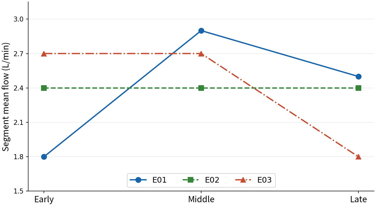
The vertical axis is segment mean flow; the horizontal axis is segment order. Lines connecting points are comparison guides, not actual sensor trajectories or equal time intervals. E01 has its highest segment mean in the middle, E02 has three equal means, and E03 has a lower late mean than its first two segments.
E02’s horizontal line does not prove that actual flow stayed constant. Two observations of 1.40 and 3.40 also average 2.40. Their internal variation differs from constant observations of 2.40 and 2.40 despite equal means. Likewise, a one-direction decrease in segment means, as in E03, does not itself establish instability or a fault.
Segment Differences and Rates Have Different Units
Define mid_minus_early = middle−early and late_minus_mid = late−middle. Both subtract mean flows, so both use L/min.
| event_id | mid_minus_early | late_minus_mid | Statement supported by the numbers |
|---|---|---|---|
| E01 | +1.10 | −0.40 | Middle exceeds early; late is 0.40 below middle |
| E02 | 0.00 | 0.00 | All three segment means are equal |
| E03 | 0.00 | −0.90 | Early and middle are equal; late is 0.90 lower |
E01’s −0.40 alone does not give a decline rate. If, as an additional assumption, representative times for the two means are ten seconds apart, their difference divided by time is −0.40/10 = −0.04 L/min/s; at twenty seconds it is −0.02. This is an average rate between summary points. Instantaneous slopes and the actual start of a decline require original timestamps and observations.
Select events whose late mean is at least pattern_change_threshold below their middle mean. The rule is late_minus_mid <= −threshold. Among these three events, 0.30 selects E01 and E03; 0.50 selects only E03. At 0.90, E03 is still included. This illustrative threshold is in L/min and is not a fault limit. Changing the selected list does not change observations.
Combine Unequal Segments with the Appropriate Weights
For a mean across all observations, weight segment means by observation counts. If E01’s means came from 2, 2, and 6 observations, the result is (2×1.80+2×2.90+6×2.50)/10 = 2.44 L/min. Equal counts give the simple mean of 2.40, but this assumption gives late greater weight.
For an overall time average, weight by duration, provided each segment mean is itself a time average. With durations of 10, 10, and 40 seconds, E01 gives (10×1.80+10×2.90+40×2.50)/60 = 2.45 L/min. This assumes the segments cover the entire action without gaps or overlap. An unweighted mean of irregularly spaced observations cannot simply be treated as a time average.
These counts and durations are separate exercise assumptions, absent from the CSV. Preserve segment counts or durations and the averaging method when passing summaries along, so an overall mean can be recomputed for its purpose.
Read Extreme Values Alongside the Median
So far we examined segment order within one action. Now suppose five different actions have mean flows of 2, 2, 2, 2, 12 L/min. Their mean is 20/5 = 4, although most values are 2.
The median is the middle value after sorting. For five values, it is the third value, 2; for an even number, average the two central values. Replacing the maximum 12 with 22 changes the mean to 30/5 = 6 while the median remains 2. Reading both shows how a large value influences the overall level summary.
Keeping only the median and ignoring 12 or 22 is also insufficient. Inspect original records to determine whether the large value is a real event or a recording error, and retain count and maximum too. This compares a distribution across actions; it does not recover time order within an action.
Finally, correct “E01 and E03 both average 2.40, so they are the same action.” One answer is: “Their unweighted segment means agree, but middle−early is +1.10 for E01 and 0 for E03; late−middle is −0.40 versus −0.90. Overall time averages and fault status need further evidence.”
Checklist
- Can you calculate 2.40 for E01–E03 and explain their differing segment changes?
- Can you distinguish flat segment means from constant observations within segments?
- Can you distinguish differences in L/min from rates in L/min/s?
- Can you calculate 2.44 and 2.45 using segment counts and durations respectively?
- Can you explain what the five-action mean of 4 and median of 2 each show?
- Do you avoid equating pattern-rule selections with instability or faults?
Sources and Further Reading
- NIST/SEMATECH, Measures of Location. Supports mean and median definitions and their differing responses to extreme values. The CSV, graph, weighted-mean calculations, and threshold exercise are our fictional examples. / Accessed: 2026-09-19