P4-10.1 Intuition For Linear Regression¶

Section ID: P4-10.1 Version: v2026.07.20

In P4-9.2, the discussion used tuning and validation cost to ask how should promising settings be compared? Now it is time to connect that comparison procedure to one actual algorithm.

The reason this Part begins with linear regression is straightforward. Linear regression is both the most basic starting point for a regression problem and the model that shows the relationship between input and output most transparently through a slope and an intercept.

The central question of this Section is the following.

How can a model express the relationship that output tends to increase or decrease as input increases in the simplest possible way?

Linear regression answers this question first with a line.

This Section explains the basic meanings of regression, linear regression, coefficient, and intercept. Later Sections continue the surrounding judgment from this handle, and the basic sense of reading a continuous prediction with a line reconnects through this Section and the concept glossary.

Scope Of This Section¶

This Section answers the following questions.

• What kind of problem does regression handle?
• Why is linear regression described as expressing a relationship with a line?
• How can direction and size between an input feature and an output target be read?
• Why is linear regression the first algorithm studied in Part 4?

This Section first closes linear regression as the most basic regression model that first explains the relationship between input and output with a line, and focuses on holding the basic handle for reading coefficients and intercepts.

The questions that will not be widened immediately in this Section are also clear. Evaluation metrics and residual interpretation continue immediately in the next Section, P4-10.2. Basic reading of multicollinearity, hypothesis testing, and regression diagnostics is reorganized again in the supplementary learning of P4-10.3. The broader perspective on regularization and related hyperparameters reconnects again through P4-9.1 and P4-9.2.

The statistical properties of residuals, a rigorous derivation of ordinary least squares, and detailed comparison among evaluation metrics such as R², MAE, and RMSE go beyond the direct scope of this Section, so they are not treated in detail here.

Goals Of This Section¶

• You can explain regression as a problem that predicts a continuous value.
• You can describe linear regression as a model that first approximates the relationship between input and output with a line.
• You can explain that linear here means the whole input is read as one weighted sum.
• You can explain the intuition of a slope and an intercept.
• You can explain at an introductory level what linear regression tries to reduce.
• You can understand why linear regression is both a good baseline and a good starting point.

Learning Background¶

Earlier in Part 4, the discussion organized data splitting, baselines, tuning, and evaluation criteria first. The reason was to help the reader first read what problem is being solved in what form instead of memorizing algorithm names from the start.

In this curriculum, linear regression plays the following role.

In other words, linear regression comes first not because it is the easiest algorithm, but because it is the algorithm that explains the relationship between input and output most clearly.

Main Learning Content¶

What Kind Of Problem Does Regression Handle?¶

Regression does not predict a category like classification does. Instead, it predicts a numeric value that changes continuously.

Examples include the following.

The common point in these problems is that the output is a number, not yes or no.

Regression is the problem of estimating one continuous value from an input.

Why Does Linear Regression Express The Relationship With A Line?¶

The linear-model documentation of scikit-learn describes linear regression as a family of models that learn the relationship between observed values and a linear combination. This Section rewrites that idea into an easier question.

If the input increases a little, by how much does the output increase on average?

The simplest formula that answers this question has the following form.

• x: input
• y: prediction
• w: coefficient
• b: intercept

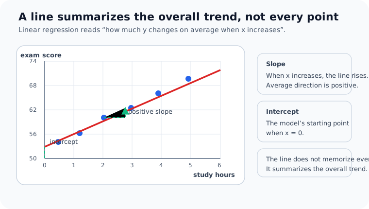
The coefficient w means how much y changes when x changes by 1. The intercept b is the starting point that the model places when the input is 0.

Seen on coordinates, this intuition becomes clearer. Even when data points do not line up perfectly on one line, linear regression finds a line that summarizes the overall direction of those points most economically. Here, the coefficient means how much it rises as it moves to the right, and the intercept means the starting point the model places when x = 0.

If that structure is read like a diagram, it becomes the following.

flowchart TD
  A["input x<br/>study hours"]
  B["coefficient w<br/>change per 1 hour"]
  C["intercept b<br/>starting point"]
  D["prediction y<br/>exam score"]

  A --> B
  B --> D
  C --> D

This diagram shows one-variable linear regression as a structure in which one input passes through a coefficient and an intercept to reach a prediction. The first point to hold here is that linear regression is not a model that memorizes data. It is a model that reads in numbers how a change in the input pushes the output upward or pulls it downward.

The key point is that linear regression does not claim that reality is perfectly a line. Rather, it asks is there a relationship that can first be explained with a line?

However, one more point should be fixed more accurately here. Readers often remember linear regression only as a model that always draws one line on a two-dimensional graph. That memory is correct for a one-variable example, but it is too narrow to explain the algorithm itself.

What Exactly Does Linear Mean?¶

The word linear in linear regression is often introduced first through the image of a line, but in theory it is closer to the idea that inputs are read as a sum with weights.

When there is one input, the form is

When there are several inputs, it expands as follows.

In other words, linear regression places one coefficient on each input feature and creates the final prediction by adding up their contributions.

Linear regression is a model that assigns one numeric contribution to each input and adds those contributions together to produce one prediction.

If this is drawn simply, it becomes the following.

flowchart TD
  A["feature x1<br/>size"]
  B["feature x2<br/>distance"]
  C["feature x3<br/>age"]
  D["weighted sum<br/>w1x1 + w2x2 + w3x3"]
  E["intercept b"]
  F["prediction y<br/>price"]

  A --> D
  B --> D
  C --> D
  D --> F
  E --> F

This diagram shows that even when the number of inputs increases, the core structure of linear regression stays the same. Even if each feature has its own meaning, the model ultimately gathers them into one weighted sum to produce a single prediction. That is the central intuition of the word linear.

So, in a one-variable example, the reader sees a line. With two or more variables, the reader moves on to a plane or a higher-dimensional linear relationship. The reader does not need to master all the mathematics of dimensionality here. It is enough to keep the point that even when inputs increase, the structure is still a weighted sum.

Why Is The Assumption Of A Line Useful?¶

Most real-world data do not sit exactly on one perfect line. Even so, linear regression still matters for three reasons.

1. It allows the simplest explanation to be tried first.
2. The coefficient and intercept are relatively easy to interpret.
3. It provides a reference point for deciding whether a more complex model is truly needed.

For example, if test scores tend to rise as study time rises, linear regression first summarizes that relationship with the question when study time increases by one hour, how many points does the score change on average?

Even if that line is not perfect, it still lets the reader answer questions like the following right away.

• Is the direction of the relationship positive or negative?
• Is the size of the change large or small?
• Is there a pattern that this simple summary misses?

In other words, linear regression is not mainly a tool that contains all of reality. It is closer to the first coordinate axis for reading reality.

What Does Linear Regression Learn?¶

In an algorithm chapter, the intuition it reads with a line is not quite enough. The reader also needs to fix what the model actually learns.

Linear regression creates predictions for data points and adjusts the coefficient and intercept so that the overall difference between those predictions and the actual values becomes small.

For each data point, this creates

• an actual value
• a prediction
• and the difference between them, called a residual or error

Linear regression chooses the line in a direction that keeps these differences from becoming too large overall.

LinearRegression in scikit-learn uses a solution corresponding to ordinary least squares by default. That flow can be read immediately through the following sentence.

A method that tries to find the line that leaves the least prediction error across the whole dataset

At this stage, what matters is not a rigorous proof or matrix calculation. The key point is that the line is chosen not by drawing a line that looks good, but by using a criterion that reduces error.

If this flow is drawn as simply as possible, it becomes the following.

flowchart TD
  A["data points"]
  B["make a trial line"]
  C["compare prediction and actual"]
  D["reduce overall error"]
  E["choose a better line"]

  A --> B --> C --> D --> E

This diagram shows that linear regression is not merely drawing a line. It is a process of searching for a better line under a criterion that reduces error. That means the heart of the algorithm is not the visible shape of the line, but how the model tries to reduce the difference between prediction and reality overall.

So linear regression is both a model that draws a line and a model that reduces error. The word algorithm becomes clearer especially from this second point of view.

When Is It Good To Raise Linear Regression First?¶

Linear regression is often a good starting point not because it is the simplest regression model, but because it is often the clearest first model for reading the direction and size of a relationship.

The key point of this table is not that linear regression is always the right model, but that it is often the first comparison model that reveals the structure of the problem.

Detailed Learning Content¶

What Misunderstandings Happen Most Often In Interpretation?¶

In linear regression, mistakes happen more often in interpretation than in formulas. The following three are especially common.

1. A Large Coefficient May Be Mistaken For An Automatically Important Feature¶

Even if the coefficient is numerically large, that does not automatically mean the feature is more important.

That is because the size of the coefficient is affected by the scale and measurement unit of the input.

• If the input is time, one unit means one hour.
• If the input is currency, one unit may mean one dollar or one won.
• If the input is distance, one unit may mean one kilometer.

So when features use different units, interpretation can become unstable if the reader compares only the raw coefficient numbers.

A coefficient is especially useful for reading direction. To compare size, unit and preprocessing must be checked together.

2. A Positive Coefficient May Be Mistaken For A Cause¶

What linear regression first shows is a tendency to move together. That does not itself mean causality.

For example, even if ad spending and sales increase together, that number alone does not prove that increasing ad spending is the only cause of higher sales.

Other explanations may still exist in between, such as

• a seasonal effect
• a promotion period
• prior brand recognition
• or an unmeasured outside variable

So the coefficient of linear regression is first an interpretive tool that shows direction and size of a relationship. It is not a tool that automatically proves a cause.

3. A Prediction May Be Read As If It Were The Actual Value¶

The output of linear regression is not a perfect copy of the world. It is an estimate obtained under the current data and the current assumptions.

For example, if the output says 7 study hours -> predicted score 76.4, that does not mean

• the person will definitely receive exactly 76.4 points

It means

• under the currently learned line, a value near that point is expected

This distinction prepares the reader to read residuals and error in the next Section.

What Assumptions Does Linear Regression Place Implicitly?¶

When studying an algorithm, it is important to build the habit of first asking how does this model simplify the world? before asking only about performance. Linear regression makes the following simplifications.

1. The Relationship Is Roughly Linear¶

It assumes that when the input changes, the output also moves in a roughly consistent direction and proportion.

For example, scores may rise as study time rises, but in reality the amount of increase may shrink after a certain point. Even so, linear regression first summarizes the overall direction with one line.

2. The Influence Of Each Input Can Be Added¶

When several features exist, linear regression first views them not as complex interactions, but as the sum of each feature's contribution.

For example, in a housing-price problem, if size, distance, and age all matter, linear regression first reads the final price as the sum of how much each element contributes.

3. Error Remains As The Unexplained Part¶

The model cannot explain every fluctuation of reality. Linear regression leaves the unexplained difference as error and places the model so that this error becomes small overall.

These three points do not explain every rigorous statistical assumption. Still, they are the key criteria for understanding the worldview of linear regression.

Linear regression is a model that simplifies relationships into a sum with one direction and treats the remaining difference as error.

Why Is Linear Regression A Good First Baseline?¶

Linear regression is often used as a baseline model because of its interpretability and simplicity.

Before trying a more complex model, running linear regression first lets the reader check the following.

• Can a simple linear relationship already explain some part of the problem?
• Do the directions between feature and target match what was expected?
• How necessary is a more complex model?

So linear regression is useful not only as a model aimed at high performance, but also as a reference model that first tests how linearly the problem can be read.

Linear regression is also especially useful for training interpretation. More complex models may achieve somewhat higher performance, but in many cases it becomes difficult to explain directly why a certain prediction appeared. Linear regression, by contrast, answers the following questions relatively directly.

• In what direction did the model read the relationship?
• As which inputs increase, does the prediction also increase?
• Is the problem too rough to be explained well by one line?

In other words, linear regression is not only the starting point of performance but also the starting point of interpretation.

This comparison also connects to later algorithm chapters.

• In P4-11 logistic regression, the line will be read again as a probabilistic classification boundary.
• In P4-14 decision trees, the relationship will be read through branching rules instead of a line.
• In P4-15 random forests, several trees will be combined to handle nonlinear relationships.

Cases And Examples¶

Case 1. How Can The Claim That Sales Rise When Ad Spending Rises Be Expressed In The Simplest Way?¶

A small online-shopping team wants first to read the relationship between monthly advertising spend and sales. The criteria people first used were questions such as in months when ad spending rises, does the number of orders also rise? and does a similar flow still appear in ordinary months without special events?

At that point, the team tries the simplest linear regression before a complex model. This is because a single line can first summarize how much sales move on average as ad spending rises, letting the reader immediately read whether the direction is positive or negative and how large the change roughly is. Reality may not be a perfect line, but as a first reference point for what change is made on average by one unit of increase, the model is already useful enough.

In this scene, linear regression is not a model that declares reality is a line. It is a model that asks can the relationship first be explained by a line? If ad spending and sales move mostly in the same direction, the coefficient and intercept become the first explanation that shows that relationship most transparently.

The confirmable result appears in the learned line and the interpretation of the coefficients. If the coefficient is positive, the reader can read the tendency that ad spending and sales increase together. If the difference between prediction and actual value is also inspected, the reader can immediately see how rough it is to explain the whole situation with one line.

flowchart TD
  A["monthly ad spend and sales"]
  B["fit one straight line first"]
  C["read slope direction and size"]
  D["compare predicted and actual points"]
  E["decide whether the linear summary is a useful first explanation"]

  A --> B --> C --> D --> E

Cases And Examples¶

Reading One-Variable Linear Regression In The Simplest Way¶

Consider an example of study time and exam score.

Looking at this data, the score does not rise by a perfectly fixed amount every time, but in general the score rises as time increases. Linear regression looks at this scene and tries to find one line such as the following.

A line in which exam scores rise on average as study time rises

What matters here is not a line that passes through every point exactly, but a line that explains the overall direction most reasonably. As discussed just above, linear regression chooses a better line under a criterion that reduces the difference between prediction and reality, and then uses that result again for predicting new inputs.

If this expression is rewritten a little more theoretically, it becomes the following.

• Some error may remain for each individual data point.
• But across the whole dataset, some lines leave smaller error and some lines leave larger error.
• Linear regression chooses the line that reduces overall error better.

In other words, linear regression is not a model that matches each individual point perfectly. It is a model that summarizes the overall tendency most economically.

How Should The Coefficient And Intercept Be Read?¶

When first learning linear regression, many readers see the formula but miss the meaning. This Section fixes interpretation before calculation.

Coefficient¶

The coefficient shows in what direction and by how much the output changes when the input changes.

• coefficient > 0: the output tends to increase as the input increases
• coefficient < 0: the output tends to decrease as the input increases
• large coefficient magnitude: the output changes more sensitively as the input changes

For example, if sales are expected to increase by about 3 units on average whenever ad spend increases by 1 unit, the coefficient can be read roughly as +3.

Still, interpretation should always keep two things together.

• direction: does the relationship increase or decrease?
• unit: what does one unit of the input actually mean?

For instance, whether the input unit means one hour of study or ten thousand won of ad spend completely changes the meaning of the same number 3. So the coefficient should be read not mainly through the number alone, but through the sentence when what changes by 1 unit, how much does what else change?

Intercept¶

The intercept is the starting point that the model places when the input is 0. However, the intercept is not always easy to interpret in reality.

For example, predicting a score when study time is 0 can still be read to some degree within the context. But interpreting a house price when the house size is 0 square meters may have little real-world meaning.

So the intercept should be read as follows.

It is the mathematical starting point of the model, but the direct interpretability depends on the domain.

Practice And Example¶

A Small Linear Regression Example In Python¶

The example below is a very small linear-regression practice that predicts exam score from study_hours.

• problem situation: roughly predict a score from study time
• input: study time
• label: actual exam score
• concepts to check:
• linear regression learns one line
• coef_ is the coefficient and intercept_ is the starting point
• the model can create a continuous-value prediction for a new input

 1
 2
 3
 4
 5
 6
 7
 8
 9
10
11
12
13
14
15
16
17
18

# This example checks linear regression slope, intercept, predictions, and residuals with NumPy calculations.
import numpy as np
from sklearn.linear_model import LinearRegression

study_hours = np.array([1, 2, 3, 4, 5, 6]).reshape(-1, 1)
exam_score = np.array([52, 55, 61, 64, 68, 72])

model = LinearRegression()
model.fit(study_hours, exam_score)

pred_2 = model.predict([[2]])[0]
pred_7 = model.predict([[7]])[0]

print("sample count      :", len(study_hours))
print("coefficient       :", round(model.coef_[0], 3))
print("intercept         :", round(model.intercept_, 3))
print("prediction at x=2 :", round(pred_2, 3))
print("prediction at x=7 :", round(pred_7, 3))

An example output is the following.

1
2
3
4
5

sample count      : 6
coefficient       : 4.114
intercept         : 47.6
prediction at x=2 : 55.829
prediction at x=7 : 76.4

This result can be read as follows.

• A coefficient of about 4.114 means that when study time increases by one hour, the score tends to rise by about four points on average.
• An intercept of about 47.6 is the mathematical starting point that the model places.
• The prediction for x=7 shows that the model can create a continuous-value prediction even for a new input that was not part of training.

What matters here is not yet exactly how many points were right, but whether the direction and size of the relationship were read with a line.

If the interpretation is written a little more carefully, it becomes the following.

• In this example, the model read a direction in which the score rises as study time increases.
• But that does not mean every interval must have exactly the same amount of increase.
• The predicted value 76.4 means the current line model estimates this value, not that the real score must certainly be exactly that number.

So the first interpretation of linear regression is not a precise prophecy of the future. It is a simple summary of a relationship.

Python Example: Reading Several Coefficients Together¶

A one-variable example is good for learning the intuition of a line, but real work data usually have several features. The example below is a small multivariable linear-regression practice that predicts final_score from three features: study_hours, attendance, and assignment_score.

• problem situation: predict a final score from study time, attendance, and assignment score together
• input: three numeric features
• label: final score
• concepts to check:
• linear regression places one coefficient on each feature
• the sign of each coefficient helps read direction
• the size of each coefficient must be read carefully together with units

 1
 2
 3
 4
 5
 6
 7
 8
 9
10
11
12
13
14
15
16
17
18
19
20
21
22
23
24
25
26
27
28

# This example checks linear regression slope, intercept, predictions, and residuals with NumPy calculations.
import numpy as np
from sklearn.linear_model import LinearRegression

X = np.array([
    [2, 80, 60],
    [3, 82, 65],
    [4, 85, 70],
    [5, 88, 72],
    [6, 90, 78],
    [7, 93, 83],
])

y = np.array([58, 63, 67, 71, 77, 82])

feature_names = ["study_hours", "attendance", "assignment_score"]

model = LinearRegression()
model.fit(X, y)

new_student = np.array([[5, 89, 75]])
pred_new = model.predict(new_student)[0]

print("sample count :", len(X))
for name, coef in zip(feature_names, model.coef_):
    print(f"{name:17}: {coef:.3f}")
print("intercept         :", round(model.intercept_, 3))
print("prediction new    :", round(pred_new, 3))

An example output is as follows.

1
2
3
4
5
6

sample count : 6
study_hours      : 2.174
attendance       : 0.609
assignment_score : 1.130
intercept         : -6.391
prediction new    : 73.12

This result can be read in the following way.

• Since the coefficient of study_hours is positive, if other conditions stay the same, the predicted score rises as study time rises.
• Since attendance and assignment_score are also positive, all three features in this example are reflected in the direction of raising the score.
• But the reader should not jump from 2.174 and 0.609 directly to the conclusion that study time is more than three times as important as attendance. The units and distributions of the two features may differ.
• A negative intercept does not mean real scores are negative in reality. This too should be read as the mathematical starting point of the model.

This multivariable example shows linear regression again as the following.

A model that reads the influence of several features separately and then adds those influences to make one prediction

Change One More Value: What Stays The Same And What Changes When One Input Goes Up?¶

Now keep attendance and assignment_score fixed for the same student and raise only study_hours from 5 to 7.

 1
 2
 3
 4
 5
 6
 7
 8
 9
10
11
12
13
14
15
16
17
18
19
20
21
22
23
24
25
26
27

# This example checks linear regression slope, intercept, predictions, and residuals with NumPy calculations.
import numpy as np
from sklearn.linear_model import LinearRegression

X = np.array([
    [2, 80, 60],
    [3, 82, 65],
    [4, 85, 70],
    [5, 88, 72],
    [6, 90, 78],
    [7, 93, 83],
])

y = np.array([58, 63, 67, 71, 77, 82])

model = LinearRegression()
model.fit(X, y)

student_base = np.array([[5, 89, 75]])
student_more_hours = np.array([[7, 89, 75]])

pred_base = model.predict(student_base)[0]
pred_more_hours = model.predict(student_more_hours)[0]

print("prediction at [5,89,75] :", round(pred_base, 3))
print("prediction at [7,89,75] :", round(pred_more_hours, 3))
print("difference              :", round(pred_more_hours - pred_base, 3))

An example output is as follows.

1
2
3

prediction at [5,89,75] : 73.12
prediction at [7,89,75] : 77.468
difference              : 4.348

What Stays The Same And What Changes?¶

• What stayed the same: when other features are fixed, the direction of the study_hours coefficient remains the same. As study time rises, the predicted score also rises.
• What changed: only one input changed, but the predicted value rose by about 4.348 points. In other words, linear regression lets the reader understand a change through the intuition of amount of input change x coefficient.
• Judgment to leave first: this change is an estimated change produced by the current model. It is not a guarantee that reality will rise by the same amount. The units and the data range still need to be checked together.

This practice rereads linear regression not as a model that memorizes a line, but as a starting point for reading in what direction and by what size the prediction moves when one input is changed. What matters in Part 4 is not only knowing the names of coefficients, but being able to change one value and explain what stayed fixed and what moved. Only with that repeated practice can later steps such as baseline comparison, residual interpretation, and deciding whether to add more features continue in the same language.

The Basic Order For Reading Numbers In This Section¶

In an algorithm chapter, it is easy to jump from numbers straight to performance is good or the prediction is correct. In linear regression, the numbers should be read in the following order.

1. First confirm that the current problem is regression.
2. Confirm what the input and output are.
3. Read the direction through the sign of the coefficient.
4. Read the size of change through the unit of the coefficient.
5. Check whether the intercept is meaningful in the current context.
6. Remember that the predicted value is an estimate, not the actual value itself.

The key point is that there is an order for reading numbers. Linear regression should not be trusted immediately just because it produced a calculation result. It should be read according to rules of interpretation like these.

Checklist¶

• Did you first confirm that the current problem is regression rather than classification?
• Did you understand that the output of linear regression is a continuous value rather than a category?
• Can you explain linear regression as the first interpretable baseline that approximates the relationship between input and output with a line?
• Can you explain the coefficient and intercept as meaning rather than only as symbols in a formula?
• Are you reading coefficient numbers together with units and context instead of immediately reading them as importance or cause?
• Did you remember that a predicted value is not the actual value, but an estimate produced by the current model?
• Can you explain why a line is still a useful starting point even when it is not perfect?

Sources And References¶

• scikit-learn, 1.1. Linear Models, scikit-learn User Guide, accessed 2026-06-26. https://scikit-learn.org/stable/modules/linear_model.html
• scikit-learn, LinearRegression, scikit-learn API Reference, accessed 2026-06-26. https://scikit-learn.org/stable/modules/generated/sklearn.linear_model.LinearRegression.html