P4-10.2 Evaluation And Limits Of Linear Regression¶

Section ID: P4-10.2 Version: v2026.07.20

P4-10.1 introduced linear regression as a model that first reads a relationship with a line. Now the discussion moves to the next question.

How well did that line actually fit, and from what point does it begin to fail easily?

That question is exactly the starting point of evaluation and limits.

After learning linear regression, readers often stop at statements such as the coefficient looks plausible or the predictions seem close enough. In an algorithm chapter, however, the reader has to go one step further. The reader must inspect how to read the gap between prediction and reality, how to summarize it through metrics, and when the line assumption becomes too weak.

So this Section does not stop at a line was drawn. It reads how much that line explains the data.

This Section does not repeat the basic definition of linear regression at length. The core intuition of a model that reads a relationship with a line reconnects through P4-10.1 and the concept glossary, while this Section focuses only on evaluation and limits.

Scope Of This Section¶

This Section answers the following questions.

• How should residual and error be understood?
• What does it mean to say that a linear-regression prediction fits well?
• At an introductory level, how can MAE, MSE, RMSE, and R² be distinguished?
• What kinds of limits appear when the line assumption breaks down?
• Up to what point should a linear-regression result be trusted, and from what point should it be read more cautiously?

This Section first closes linear-regression results through the two questions how much did it fit? and from where does it begin to fail easily?, and focuses on holding residuals and evaluation metrics as the handles for that judgment.

The questions that will not be widened immediately in this Section are also clear. Basic reading of regression diagnostics, significance testing, and multicollinearity is reorganized again in the supplementary learning of P4-10.3. The broader view of regularization and related hyperparameters reconnects again through P4-9.1 and P4-9.2. The broader flow of feature engineering reconnects again through P4-7.1, P4-7.2, P4-18.1, and P4-18.2.

Statistical significance testing, rigorous tests of residual normality and homoscedasticity, multicollinearity diagnosis, and advanced regularization and feature engineering go beyond the direct scope of this Section, so they are not treated in detail here.

Goals Of This Section¶

• You can explain a residual as the difference between the actual value and the prediction.
• You can say from what angle MAE, MSE, RMSE, and R² each summarize a model.
• You can distinguish metrics that react more strongly to large errors from metrics that react less strongly.
• You can explain typical situations in which linear regression does not fit well.
• You can understand why one good-looking number is not enough to overtrust linear regression.

Learning Background¶

P4-10.1 introduced linear regression as the first model that summarizes a relationship. But once a model is set up, the next step must be to read how much it actually fit.

• Even when there is a line, prediction error still remains.
• If error remains, the reader must decide how to summarize its size.
• Even if a metric looks good, the model should be questioned again if the line misses an important pattern.

This gives the Section the following role in the algorithm part of the curriculum.

If P4-10.1 was the Section that inspected the shape of the model, P4-10.2 is the Section that inspects the difference left by the model.

In regression evaluation, the following four items should be left together.

Good regression evaluation therefore does not end with a single metric. It checks together whether the model improved beyond the baseline, how much it misses on average, where it misses badly, and what scene that failure repeats in.

The same comparison structure from the classification chapter also continues here. In regression, a baseline may be a reference model such as a simple average prediction, or it may be a comparison line that places recent prediction error next to a typical error distribution. So even regression evaluation is not only about reading an absolute error number. It also asks whether the current error is larger than usual and whether the same failure repeats only in a certain region. Here again, large error is first read as a signal of change, and an explanation of the cause should be added only after missing features or segment differences are checked again.

So the comparison frame in regression evaluation must also stay unified. If baseline error, current-model error, and recent-region error distribution are read separately under different units or different regions, it becomes difficult to say what actually improved.

Main Learning Content¶

What Is The Difference Between Residual And Error?¶

When readers first meet the two words, they can look similar. In this book, however, they are distinguished as follows.

• residual: actual value - prediction for one individual data point
• error: a general word for the difference that the model leaves behind

For example, if the actual score is 72 and the prediction is 68, the residual is 72 - 68 = 4. If the actual score is 64 and the prediction is 67, the residual is 64 - 67 = -3.

What matters here is the sign and the size.

• positive residual: the model predicted too low
• negative residual: the model predicted too high
• large absolute value: the prediction missed more on that data point

When looking at one point, the residual is the vertical distance between the actual point and the predicted point on the regression line. So when reading residuals, it is faster to look not only at a number table but also at how far above or below the line the point sits.

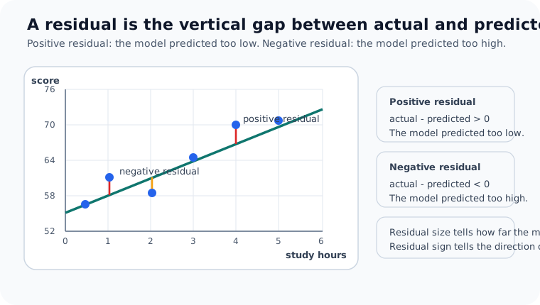
If this is drawn simply, it becomes the following.

flowchart TD
  A["actual value"]
  B["prediction"]
  C["residual = actual - prediction"]
  D["positive residual<br/>predicted too low"]
  E["negative residual<br/>predicted too high"]

  A --> C
  B --> C
  C --> D
  C --> E

This diagram helps the reader see a residual not as a flat failure mark, but as a difference that has direction. The reader has to see together whether the prediction was below or above the actual value in order to suspect later whether the model is systematically leaning to one side in a certain region.

The key point is that a residual is not simply wrong. It shows in which direction and by how much the model missed.

What Does It Mean For A Linear-Regression Prediction To Fit Well?¶

In regression, it is hard to divide outcomes directly into correct and incorrect the way classification often does. Numeric prediction usually misses by at least a little. So when the reader reads a regression model, the first question is not how often did it match exactly? but how far does it miss on average?

Suppose there are two models.

Both can look plausible on average, but in actual use B may be more dangerous. That is why regression evaluation centers on how the error is summarized.

So in regression, the sentence it fits well usually has to be unpacked into the following questions.

• How far does it miss on average?
• Are there frequent large errors?
• Is it actually better than the baseline?
• Is there a structural pattern that the line misses?

How Should MAE, MSE, And RMSE Be Distinguished?¶

The regression-metric documentation of scikit-learn provides metrics such as mean absolute error, mean squared error, and R². At the introductory level, the reader understands them more easily through what kind of mistake each metric punishes more strongly than through formulas alone.

MAE¶

MAE averages the absolute values of residuals.

• It is easy to interpret.
• It is easy to read as on average, the prediction misses by about how many points, minutes, or units.
• It does not especially exaggerate large errors.

So MAE is the metric that shows most plainly how much the model misses on average.

MSE¶

MSE squares the residuals and then averages them.

• It reacts more strongly to large errors.
• It weighs a few large misses more heavily than several small ones.
• It can be less intuitive to interpret because the unit is squared.

So MSE is useful when the reader wants to punish large mistakes more strongly.

RMSE¶

RMSE takes the square root of MSE.

• It keeps the advantage of reacting strongly to large errors.
• It returns to the original unit, so interpretation becomes easier again.

So RMSE is often used when the reader wants to remain sensitive to large errors but still read the result in the original unit.

The difference can be summarized very briefly as follows.

In a work scene, the difference becomes even clearer.

So metric choice is not a matter of mathematical taste. It connects directly to what kind of mistake hurts more.

What Does R² Show?¶

R² is a familiar number in introductory linear regression, but it is also easy to misunderstand.

R² is a summary value that shows how much more this model explains the data than a simple average prediction does.

At an introductory level, the reader can interpret it as follows.

• close to 1: the line explains quite a lot of the variation in the current data
• close to 0: it is not very different from predicting with the average
• can even be negative: it can be worse than an average prediction

The important point is that R² is easily misread as a simple score that is always better when higher. But R² alone cannot reveal whether a few large errors are hiding underneath. So it must be read together with error metrics such as MAE and RMSE.

Scenes like this also appear often in practice. For example, in sales prediction, most ordinary weekdays may be predicted well, but the model may fail badly on a few large event days. In that case, the line may explain a large share of overall variation, so R² may still look high, but an operator may still find the model hard to trust because of those few large failures.

So R² is strong at showing overall explanatory power, but it does not replace the lived impact of a few large failures.

How Should Metrics Be Read Together?¶

When linear regression is read through only one metric, interpretation can become unstable. The following scenes are typical.

Regression evaluation becomes clearer when it is read in the following order.

1. Did the model improve beyond the baseline?
2. How large is the average error?
3. Are there any unusually large errors?
4. Are residuals leaning repeatedly in one direction?

If this order is drawn simply, it becomes the following.

flowchart TD
  A["compare with baseline"]
  B["check average error<br/>MAE or RMSE"]
  C["check large misses"]
  D["look for residual pattern"]

  A --> B --> C --> D

This diagram organizes the order in which regression metrics should be read. Good regression evaluation is not the act of reading one number. It is the act of checking in sequence whether the model beat the baseline, how large the average error is, and whether large failures are hiding.

The main point is not to stop at one number looks good.

Regression evaluation records should also keep the following three sentences together.

• A change is visible, but the cause is not fixed yet.
• A region with large error is a signal that review priority should be raised.
• A large error in a small-sample segment should be interpreted more conservatively.

These three sentences point to the same overall lesson. Regression evaluation also becomes more explainable when it reads not one error number, but the same baseline, the same region, and the same representative failure side by side.

Which Metric Should Be Read First?¶

Rather than listing regression metrics all at once, the reader should make the reading order explicit based on what kind of failure needs the most attention right now.

The purpose of this table is not to lock the reader into one metric, but to make the evaluation order clear according to what kind of failure is being read right now.

Detailed Learning Content¶

What Typical Situations Make Linear Regression Fit Poorly?¶

The limits of linear regression usually appear when one line is not enough, but the model is still pushed to explain everything with one line.

Typical scenes include the following.

1. When The Relationship Is Nonlinear¶

As the input grows, the output may rise quickly at first and then become flatter after some point. In that case, one line struggles to fit the early and late segments together.

A familiar example is a case in which score keeps rising as study time rises, but the size of the increase becomes smaller after a certain amount of study time.

2. When The Relationship Changes By Region¶

Some data change character before and after a certain region.

• the price structure for small houses can differ from that for large houses
• the time pattern for short delivery distance can differ from that for long distance

When such a dataset is summarized by one line, the result can look plausible on average but still keep failing inside each region.

3. When An Important Feature Is Missing¶

Sometimes the problem is not the line itself, but the fact that a feature needed for explanation is missing.

For example, if house-price prediction uses size but leaves out location, the model may appear to read the relation between size and price while actually missing an important structure.

4. When Outliers Are Strong¶

Linear regression cannot simply ignore large errors. If a few data points lie unusually far away, the line can be pulled toward them and the overall interpretation can become unstable.

Typical practical scenes include the following.

• delivery time usually stayed between 5 and 20 minutes, but one storm day produced 90 minutes
• sales usually stayed between 20 and 60 million won, but one event produced 2 billion won
• a few ultra-expensive penthouses are mixed into otherwise ordinary housing-price ranges

Such points may represent important real events, but when one line is used to read the whole dataset, they can pull the model too strongly.

So the limit of linear regression should be read less as the algorithm is bad and more as summarizing the current problem with only one line may be too much.

The most typical first suspicions are the true relationship is actually curved and a few extreme values are pulling the line.

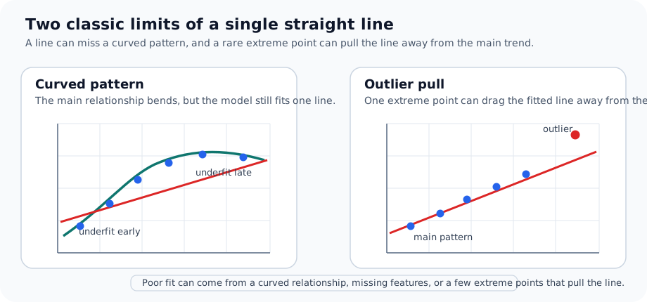
That signal can be shortened into a practical retrospective note as follows.

Supplement To The Detailed Learning Content¶

Academic Background And History¶

Once evaluation and limits have been read, it becomes easier to understand why linear regression reads error in this way. There are two historical streams behind it.

The first is the stream of least squares. The problem of choosing a line or formula that best explains data with observation error was very important in early nineteenth-century astronomy and geodesy. In that context, least squares quickly became established as a method for systematically reducing observational differences.

The second is the stream behind the name regression itself. The word became widely known through Francis Galton's work on heredity and height in the late nineteenth century. At that time it described the tendency of extreme values to move back toward the average in the next generation, and later widened into the name of general linear-relation estimation in statistics.

• least squares came from the history of a computational method that reduces error
• regression came from the history of a statistical interpretation that tries to quantify relationships
• today's linear regression is the result of these two streams being combined

With that background, it becomes clearer that linear regression is not only the first algorithm in a textbook. It is the meeting point between a way of handling observation error and a way of interpreting relationships.

Where Do The Main Disputes Arise?¶

Only after metrics and limits have been read can the disputes around linear regression be read more accurately. Linear regression itself is an old classical tool, but disputes about interpretation still repeat today. Four especially important ones are the following.

1. Treating Prediction And Explanation As If They Were The Same Sentence¶

Even if a regression formula predicts quite well, its coefficient cannot automatically be taken as an explanation of the real-world cause. Having predictive performance and explaining causality are different issues.

This dispute appears often in data-driven services too.

• good sales prediction does not mean the ad-spend coefficient proves causal effect
• good house-price prediction does not mean one specific variable determines price

So linear regression helps interpretation, but it does not automatically prove causality.

2. Reading The Coefficient Directly As Importance¶

A large coefficient does not directly mean that a feature is more essential. Scale, preprocessing, and feature-selection procedure all influence it together.

This dispute is especially common in multivariable regression. When reading coefficients, the reader should ask not first is it large or small? but under what unit was it measured?

3. Overtrusting A High R²¶

When R² is high, the model looks as if it explains the data well. But a few large failures, a structural error in one region, or missing important variables can all hide underneath a high R².

So R² is a useful summary value, but not a final verdict.

4. The Gap Between The Historical Origin Of Regression And Social Interpretation¶

The word regression spread widely together with Galton's heredity research, and around it there was also a history of determinism and eugenics that is critically reexamined today. When learning linear regression in modern statistics and machine learning, the reader should separate the mathematical tool itself from the social interpretations attached to it at the time.

This is a different kind of dispute from technical limits, but it still shows that explaining relationships with numbers does not automatically justify the social meaning attached to those explanations.

Good And Bad Readings Of Linear Regression¶

Linear regression has the advantage of high interpretability, but because of that it is also easy to produce hasty interpretation.

The especially important sentence is the following.

Linear regression helps interpretation begin, but it does not finish interpretation for us.

Cases And Examples¶

Case 1. Delivery-Time Prediction That Looks Fine On Average But Fails Badly In A Specific Customer Region¶

A logistics team is predicting arrival time from delivery distance and order time band. The criteria people first watched were relationships such as does a longer distance really take more time? and do evening orders tend to arrive later?

When the team runs linear regression, the overall R² is fairly high and MAE is not bad either. On the surface, the model can look acceptable. But when inspected more closely, predictions miss badly on long-distance deliveries or days with heavy rain, and RMSE becomes higher than expected because of those large failures.

flowchart TD
  A["delivery time data"]
  B["linear regression"]
  C["compare with baseline"]
  D["check MAE for average miss"]
  E["check RMSE for large misses"]
  F["inspect residuals by route and weather"]
  G["decide whether linear fit is enough"]

  A --> B --> C --> D
  D --> E --> F --> G

In this scene, regression evaluation does not end with one number. MAE shows how much the model misses on average, RMSE reacts more strongly to rare large failures, and R² summarizes the size of overall explanatory power. So R² is high alone cannot explain the real operational risk.

The confirmable result appears when residuals and metrics are read together. Even if average error looks small, if residuals cluster strongly to one side in a certain region or large failures keep repeating, the reader should treat that as a signal that linear regression is not explaining the structure of that region well enough. Even this difference should first be read as a review-priority signal that says what region must be inspected next, not as a sentence that fixes the cause automatically.

Empirical Example 1. Delivery-Time Prediction¶

Suppose a team is predicting delivery time for the same region.

If the reader looks only at the average number, B can look better. But if some customers experience delays of 30 or 40 minutes, the actual service experience may be worse instead.

That means the empirical example shows why MAE and RMSE must be read together.

Empirical Example 2. Housing-Price Prediction¶

In housing-price prediction, the model may fit most middle-price houses well but fail badly on very expensive houses.

• MAE can still be fairly low.
• RMSE can become higher because of the large errors on high-priced homes.
• R² can still look high because the overall variation is explained reasonably well.

The important question in this scene is not only is it acceptable on average? It is in what region is it especially risky?

So metrics show the overall average, but a practical reading is only complete when the failure pattern by region is also checked.

Practice And Example¶

Looking At Residuals And Metrics Together In Python¶

The example below reuses the study-time data from 10.1 and checks prediction, residuals, MAE, RMSE, and R² together.

• problem situation: after predicting exam score from study time, check how much the model missed
• input: study time
• label: actual exam score
• concepts to check:
• residuals are created separately for each data point
• MAE and RMSE summarize error
• R² shows how much more the model explains than an average prediction

 1
 2
 3
 4
 5
 6
 7
 8
 9
10
11
12
13
14
15
16
17
18
19

# This example calculates residuals and evaluation metrics such as MAE, MSE, and RMSE for linear regression predictions.
import numpy as np
from sklearn.linear_model import LinearRegression
from sklearn.metrics import mean_absolute_error, mean_squared_error, r2_score

study_hours = np.array([1, 2, 3, 4, 5, 6]).reshape(-1, 1)
exam_score = np.array([52, 55, 61, 64, 68, 72])

model = LinearRegression()
model.fit(study_hours, exam_score)

pred = model.predict(study_hours)
residuals = exam_score - pred

print("predictions :", np.round(pred, 3))
print("residuals   :", np.round(residuals, 3))
print("MAE         :", round(mean_absolute_error(exam_score, pred), 3))
print("RMSE        :", round(mean_squared_error(exam_score, pred) ** 0.5, 3))
print("R2          :", round(r2_score(exam_score, pred), 3))

An example output is as follows.

1
2
3
4
5

predictions : [51.714 55.829 59.943 64.057 68.171 72.286]
residuals   : [ 0.286 -0.829  1.057 -0.057 -0.171 -0.286]
MAE         : 0.448
RMSE        : 0.608
R2          : 0.992

This output can be read as follows.

• Residuals contain both positive and negative values, so the model is not strongly missing only in one direction.
• MAE around 0.448 means the model misses by about 0.45 points on average.
• RMSE around 0.608 is an average error that reacts a little more strongly to larger misses.
• R² around 0.992 shows that, in this small example, the line explains a large share of the variation in the data.

Even here, however, there are several cautions.

• The dataset is small and simple.
• The model is being evaluated again on the same points it learned from, so this is not the same as actual generalization performance.
• A pretty-looking number does not mean linear regression is sufficient for every regression problem.

So metrics are tools that help interpretation. They are not tools that deliver a final verdict all at once.

Seeing How One Outlier Shakes Metrics In Python¶

The example below inserts a large error into the last point of an otherwise similar pattern and shows how MAE and RMSE react differently.

Problem situation:

• assume a scene where most cases follow a similar pattern, but one data point fails badly

Input:

• actual-value array actual
• ordinary prediction pred_good
• prediction pred_outlier with a large error in the last point

Expected output:

• MAE in the two cases
• RMSE in the two cases

Concepts to check:

• MAE shows the average miss
• RMSE reacts more strongly to one large failure

 1
 2
 3
 4
 5
 6
 7
 8
 9
10
11
12

# This example calculates residuals and evaluation metrics such as MAE, MSE, and RMSE for linear regression predictions.
import numpy as np
from sklearn.metrics import mean_absolute_error, mean_squared_error

actual = np.array([52, 55, 61, 64, 68, 72])
pred_good = np.array([51, 56, 60, 65, 67, 73])
pred_outlier = np.array([51, 56, 60, 65, 67, 90])

print("good MAE    :", round(mean_absolute_error(actual, pred_good), 3))
print("good RMSE   :", round(mean_squared_error(actual, pred_good) ** 0.5, 3))
print("outlier MAE :", round(mean_absolute_error(actual, pred_outlier), 3))
print("outlier RMSE:", round(mean_squared_error(actual, pred_outlier) ** 0.5, 3))

An example output is as follows.

1
2
3
4

good MAE    : 1.0
good RMSE   : 1.0
outlier MAE : 3.833
outlier RMSE: 7.431

This output is very useful for interpretation training.

• In the good prediction, MAE and RMSE are almost the same.
• In the outlier prediction, MAE also rises, but RMSE reacts much more sharply.

Seen empirically, RMSE really is the metric that dislikes large failures more.

What Stays The Same And What Changes If Large Failure Spreads To Two Points?¶

This time, instead of only the last point failing badly, change the scene so that the last two points both fail badly.

 1
 2
 3
 4
 5
 6
 7
 8
 9
10
11
12

# This example calculates residuals and evaluation metrics such as MAE, MSE, and RMSE for linear regression predictions.
import numpy as np
from sklearn.metrics import mean_absolute_error, mean_squared_error

actual = np.array([52, 55, 61, 64, 68, 72])
pred_outlier = np.array([51, 56, 60, 65, 67, 90])
pred_two_outliers = np.array([51, 56, 60, 65, 84, 90])

print("one-outlier MAE :", round(mean_absolute_error(actual, pred_outlier), 3))
print("one-outlier RMSE:", round(mean_squared_error(actual, pred_outlier) ** 0.5, 3))
print("two-outlier MAE :", round(mean_absolute_error(actual, pred_two_outliers), 3))
print("two-outlier RMSE:", round(mean_squared_error(actual, pred_two_outliers) ** 0.5, 3))

An example output is as follows.

1
2
3
4

one-outlier MAE : 3.833
one-outlier RMSE: 7.431
two-outlier MAE : 6.5
two-outlier RMSE: 8.91

What Stayed The Same And What Changed?¶

• What stayed the same: in both cases, RMSE still reacts more strongly than MAE. The interpretation it is more sensitive to large failures stays valid.
• What changed: once large failure spread from one point to two points, MAE also rose much faster. That means the signal the model is now also missing a lot on average becomes stronger.
• Judgment to leave first: the same rise in error leads to very different operational questions depending on whether it is a one-point accident or a repeated failure over several points.

What Stayed The Same And What Changed?¶

• What stayed the same: in both cases, RMSE still reacts more strongly than MAE. The interpretation it is more sensitive to large failures stays valid.
• What changed: once large failure spread from one point to two points, MAE also rose much faster. That means the signal the model is now also missing a lot on average becomes stronger.
• Judgment to leave first: the same rise in error leads to very different operational questions depending on whether it is a one-point accident or a repeated failure over several points.

The core of this comparison is to shift regression evaluation from reading numbers to reading failure structure. The real question is not simply whether the error grew, but where, at how many points, and in what direction the failure grew. More important than memorizing the difference between MAE and RMSE is training the distinction between one large failure and a repeated failure region.

The core of this Section is not memorizing more regression metric names. It is fixing how far regression evaluation should be read together.

Checklist¶

• Before confirming improvement beyond the baseline, are you drawing a conclusion from only one error number?
• Can you explain that a residual is the difference between the actual value and the prediction?
• Can you explain what the sign of a residual means?
• Can you explain the difference between MAE and RMSE through sensitivity to large errors?
• Did you understand R² not as a simple score, but as explanatory power relative to the baseline?
• Are you reading average error separately from large failures?
• Did you understand that interpretation can become unstable when only one metric is used, so baseline, average error, large error, and residual pattern must be checked together?
• When a large-error region appears, are you avoiding fixing the cause immediately and instead rechecking missing features or nonlinear possibility?
• Do you understand that the limits of linear regression usually appear in problems that are too much to summarize with one line?
• Can you give one or two examples of scenes where the line assumption breaks down?
• Can you explain why a good-looking number still should not be overtrusted immediately?

Sources And References¶

• scikit-learn, 1.1. Linear Models, scikit-learn User Guide, accessed 2026-06-26. https://scikit-learn.org/stable/modules/linear_model.html
• scikit-learn, 3.4. Metrics and scoring: quantifying the quality of predictions, scikit-learn User Guide, accessed 2026-06-26. https://scikit-learn.org/stable/modules/model_evaluation.html
• scikit-learn, mean_absolute_error, scikit-learn API Reference, accessed 2026-06-26. https://scikit-learn.org/stable/modules/generated/sklearn.metrics.mean_absolute_error.html
• scikit-learn, mean_squared_error, scikit-learn API Reference, accessed 2026-06-26. https://scikit-learn.org/stable/modules/generated/sklearn.metrics.mean_squared_error.html
• scikit-learn, r2_score, scikit-learn API Reference, accessed 2026-06-26. https://scikit-learn.org/stable/modules/generated/sklearn.metrics.r2_score.html