P4-10.3 Supplementary Learning: How To First Read Regression Diagnostics¶

Section ID: P4-10.3 Version: v2026.07.20

By the time the reader finishes P4-10.2, the basic evaluation of linear regression is in place. In actual documents and lectures, however, the reader soon meets expressions such as the following.

• statistical significance
• residual normality
• homoscedasticity
• multicollinearity

The purpose of this Section is not to learn proofs of every one of these concepts. Its purpose is to organize what kind of worry these words point to so that the reader does not stop when reading a regression-results table.

This supplementary learning does not re-explain the definition of linear regression by extending it. The basic intuition and the evaluation handles remain in P4-10.1, P4-10.2, and the concept glossary. Here the focus is only on what kinds of risk regression-diagnostic terms point to.

Scope Of This Supplementary Learning¶

This Section answers the following questions.

• Why do regression diagnostics come after linear regression?
• What should the reader watch out for when reading statistical significance?
• What kind of concern lies behind residual normality and homoscedasticity?
• Why can multicollinearity shake the interpretation of coefficients?

This supplementary learning first closes regression diagnostics through the question what kinds of risk should be checked to avoid overtrusting a linear-regression result, and focuses on recovering the interpretation-stability question left in P4-10.2.

Formula derivations of each test statistic, the full history of debates around p-value interpretation, VIF practice, and advanced regression-package usage go beyond the direct scope of this supplementary learning, so they are not treated in detail here.

Goals Of This Supplementary Learning¶

• You can explain regression diagnostics as checks that keep the reader from overtrusting a linear-regression result.
• You can distinguish what significance, normality, homoscedasticity, and multicollinearity each worry about.
• When reading a coefficient table, you can avoid treating there is a number and the interpretation is stable as the same statement.

Why Is Regression Diagnostics Treated Separately?¶

Linear regression is a model that fits a line, but drawing a line does not automatically make the interpretation safe. So regression diagnostics usually continue through questions like the following.

1. How far does this line miss on average?
2. Is that error leaning in a certain direction?
3. Are input features overlapping so much that coefficient interpretation becomes unstable?
4. Up to what point can the numbers in the coefficient table be trusted?

So regression diagnostics is not the language of performance score. It is the language of checking interpretive stability.

What Does Statistical Significance Ask?¶

Could this coefficient or relationship appear only from random fluctuation, or does it appear as a reasonably consistent signal inside the data?

The important point is that significance does not automatically mean practical importance or predictive performance.

These two can differ. So significance is one axis that asks why does this number seem to exist, but it does not replace the quality of the whole model.

What Does Residual Normality Worry About?¶

Residual normality, stated very simply, worries about whether error is becoming extremely skewed into a certain strange shape.

The reader does not need to feel that normality is an absolute condition for making predictions. But inside coefficient interpretation and some statistical-test contexts, if residual shape is strongly crushed toward one side, the interpretation can become less stable.

• when residuals stretch very far to one side, interpretation needs more caution
• one large outlier can shake the residual shape strongly

A very small comparison exercise can be read as follows.

1
2
3
4
5
6
7
8

# This example checks residual balance, outliers, and range-level error patterns for regression diagnostics.
balanced_residuals = [-3, -1, 0, 1, 3]
skewed_residuals = [-1, 0, 1, 2, 12]

print("balanced residuals:", balanced_residuals)
print("skewed residuals  :", skewed_residuals)
print("balanced range    :", max(balanced_residuals) - min(balanced_residuals))
print("skewed range      :", max(skewed_residuals) - min(skewed_residuals))

An example output is the following.

1
2
3
4

balanced residuals: [-3, -1, 0, 1, 3]
skewed residuals  : [-1, 0, 1, 2, 12]
balanced range    : 6
skewed range      : 13

This comparison does not replace a normality test, but it immediately shows the difference between a scene where error is spread in a fairly balanced way and a scene where one long tail appears on one side. At an introductory level, it is enough to read residual normality as the language that first worries about whether error stretches too far to one side and destabilizes interpretation.

What Does Homoscedasticity Worry About?¶

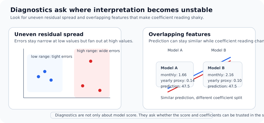
Homoscedasticity worries about whether the spread of error changes too much across input regions.

For example, if error is small in a low-value region but becomes larger and larger as the values grow, questions like the following appear.

• Is the model unusually unstable only in a specific region?
• Is there a hidden structure that is difficult to explain with just one line?

So homoscedasticity is the viewpoint that asks is the spread of error roughly similar across all regions?

A very small comparison table can be read as follows.

In such a scene, the reader should first inspect where the explanation breaks down rather than stopping at the average performance looks acceptable.

If regression diagnostics is compressed into one frame, one side asks does the spread of error change by region?, while the other asks does prediction stay similar while only coefficient interpretation shakes?

Why Does Multicollinearity Shake Coefficient Interpretation?¶

Multicollinearity appears when input features contain too much overlapping information.

For example, if strongly overlapping features such as

• monthly_spend
• quarterly_spend
• yearly_spend

enter together, the model may still predict reasonably well, but it may become hard to say stably which feature's coefficient was really more important.

The core point is the following.

Being able to predict and having stable coefficient interpretation are not the same thing.

Cases And Examples¶

Case 1. Housing-Price Prediction Seems To Fit, But Coefficient Interpretation Keeps Wobbling¶

A real-estate analysis team is building a regression formula for housing-price prediction. The human questions used first were things like does a larger area make the house more expensive?, does being closer to a station raise the price?, and does a newer home tend to be worth more?

But even if the input columns do not contain a trivial duplicate such as monthly_spend, strongly overlapping information still enters together through variables such as floor area, supplied area, number of rooms, and number of living rooms. The prediction itself can look plausible, but in one experiment the area coefficient becomes large, while in another the room-count coefficient becomes larger, and even the direction of the coefficient can become unstable. In this kind of scene, prediction performance and the stability of coefficient interpretation must not be treated as the same statement.

flowchart TD
  A["housing features"]
  B["good prediction fit"]
  C["unstable coefficients"]
  D["check overlapping features"]
  E["check residual spread"]
  F["check interpretation stability"]

  A --> B
  A --> C
  C --> D --> E --> F

At this point, regression diagnostics asks up to what point can this number be trusted? Multicollinearity can shake coefficient interpretation because similar features end up sharing explanatory roles. If homoscedasticity breaks, error can spread more widely in a specific price region. If residual shape leans to one side, interpretation should again become more cautious. So obtaining one line does not automatically make the whole coefficient table a safe explanation.

The confirmable result appears when residual distribution and feature overlap are viewed together. If prediction stays roughly similar but the size and sign of coefficients keep wobbling across experiments, that regression formula may be a model that is still usable for prediction but should be read more carefully for explanation.

Practice And Example¶

See In Python How Overlapping Features Shake Coefficient Interpretation¶

The example below shows that when two features carrying nearly the same information enter together, prediction may remain similar while coefficient interpretation wobbles.

• problem situation: read a regression formula that contains both monthly_spend and yearly_spend_proxy
• input: monthly_spend, yearly_spend_proxy
• label: next-month sales
• concepts to check:
• when strongly overlapping features enter together, coefficient roles can appear split
• keeping prediction stable and keeping coefficient interpretation stable are not the same thing

 1
 2
 3
 4
 5
 6
 7
 8
 9
10
11
12
13
14
15
16
17
18
19
20
21
22
23
24

# This example checks residual balance, outliers, and range-level error patterns for regression diagnostics.
import numpy as np
from sklearn.linear_model import LinearRegression

monthly_spend = np.array([10, 12, 14, 16, 18, 20], dtype=float)
yearly_spend_proxy = np.array([121, 145, 167, 193, 215, 239], dtype=float)
y = np.array([30, 35, 40, 45, 50, 55], dtype=float)

X_two_features = np.column_stack([monthly_spend, yearly_spend_proxy])
X_one_feature = monthly_spend.reshape(-1, 1)

model_two = LinearRegression()
model_two.fit(X_two_features, y)

model_one = LinearRegression()
model_one.fit(X_one_feature, y)

query_two = np.array([[17, 203]], dtype=float)
query_one = np.array([[17]], dtype=float)

print("two-feature coefficients :", np.round(model_two.coef_, 3))
print("two-feature prediction   :", round(model_two.predict(query_two)[0], 3))
print("one-feature coefficient  :", round(model_one.coef_[0], 3))
print("one-feature prediction   :", round(model_one.predict(query_one)[0], 3))

An example output is the following.

1
2
3
4

two-feature coefficients : [1.661 0.143]
two-feature prediction   : 47.517
one-feature coefficient  : 2.5
one-feature prediction   : 47.5

What the reader should first take from this result is the following.

• The two models make almost the same prediction.
• But when the two features enter together, coefficient interpretation gets split into 1.661 and 0.143.
• That means prediction can stay similar while which feature is really more important becomes more unstable.

What Stays The Same And What Changes If Only One Point Of An Overlapping Feature Moves?¶

This time, the reader changes only the last value of yearly_spend_proxy from 239 to 233 and trains again.

 1
 2
 3
 4
 5
 6
 7
 8
 9
10
11
12
13
14
15
16
17
18
19
20
21
22

# This example checks residual balance, outliers, and range-level error patterns for regression diagnostics.
import numpy as np
from sklearn.linear_model import LinearRegression

monthly_spend = np.array([10, 12, 14, 16, 18, 20], dtype=float)
yearly_spend_proxy = np.array([121, 145, 167, 193, 215, 239], dtype=float)
yearly_spend_shifted = np.array([121, 145, 167, 193, 215, 233], dtype=float)
y = np.array([30, 35, 40, 45, 50, 55], dtype=float)

query = np.array([[17, 203]], dtype=float)

model_original = LinearRegression().fit(
    np.column_stack([monthly_spend, yearly_spend_proxy]), y
)
model_shifted = LinearRegression().fit(
    np.column_stack([monthly_spend, yearly_spend_shifted]), y
)

print("original coefficients :", np.round(model_original.coef_, 3))
print("original prediction   :", round(model_original.predict(query)[0], 3))
print("shifted coefficients  :", np.round(model_shifted.coef_, 3))
print("shifted prediction    :", round(model_shifted.predict(query)[0], 3))

An example output is the following.

1
2
3
4

original coefficients : [1.661 0.143]
original prediction   : 47.517
shifted coefficients  : [2.157 0.097]
shifted prediction    : 47.479

What Stayed The Same And What Changed?¶

• What stayed the same: the predictions of the two models are still almost identical.
• What changed: even though only one value of an overlapping feature moved slightly, the way the coefficients were distributed shifted quite a lot.
• What judgment should be left first: in a scene like this, the reader should first recall the warning from regression diagnostics that prediction may still be usable, but coefficient interpretation must be handled more carefully.

This exercise recovers regression diagnostics not as a list of statistical terms learned later, but as a procedure that asks again how far the reader can trust the model result. What matters is not to accept a score and coefficient table as they are, but to separate cases in which prediction itself shakes from cases in which only interpretation shakes. Multicollinearity is one representative scene that forces exactly this distinction.

Read Homoscedasticity Too Through One Small Comparison¶

Instead of stopping after multicollinearity alone, the reader can compare one tiny scene where the spread of error differs by region.

1
2
3
4
5
6

# This example checks residual balance, outliers, and range-level error patterns for regression diagnostics.
low_range_residuals = [-2, 1, 0]
high_range_residuals = [-15, 12, 18]

print("low-range spread  :", max(low_range_residuals) - min(low_range_residuals))
print("high-range spread :", max(high_range_residuals) - min(high_range_residuals))

An example output is the following.

1
2

low-range spread  : 3
high-range spread : 33

This does not replace a complex test, but it immediately shows at an introductory level that even under the same regression formula, the spread of error can be much wider in one region than in another. In other words, regression diagnostics asks not only about unstable coefficient interpretation, but also about imbalance in how error spreads.

When The Small Practices In This Supplementary Learning Are Read Together¶

• the residual-normality comparison makes the reader inspect first does the error shape stretch too far to one side?
• the homoscedasticity comparison makes the reader inspect first in what region does the error spread become larger?
• the multicollinearity comparison makes the reader inspect first does prediction remain stable while only coefficient interpretation shakes?

So regression diagnostics is better read not as a chapter for memorizing one test name, but as a chapter for separating which one is wobbling among error shape, error spread, and stability of coefficient interpretation.

Checklist¶

• Did you understand that regression diagnostics is less about raising a score and more about making interpretation more cautious?
• Can you avoid treating significance and practical importance as the same statement?
• Can you explain that homoscedasticity worries about whether error size changes by region?
• Can you explain why multicollinearity can shake coefficient interpretation?
• Are you avoiding treating prediction performance and the stability of coefficient interpretation as the same statement?
• When reading a linear-regression table, are you asking not only is there a number? but also how far can this number be trusted?

Sources And References¶

• statsmodels developers, Regression diagnostics, accessed 2026-07-01.
• Gareth James, Daniela Witten, Trevor Hastie, Robert Tibshirani, An Introduction to Statistical Learning, accessed 2026-07-01.