P4-11.1 Intuition For Logistic Regression
Section ID:
P4-11.1Version:v2026.07.31
In P4-10, linear regression showed how to predict a continuous value with a line. The next step is to see how that same linear way of thinking changes when the task becomes classification.
The central question of this Section is the following.
How can we keep a linear calculation but read the output as a value between 0 and 1?
That question is the starting point of logistic regression.
The name often causes confusion. If it is called regression, why is it used for classification? The final purpose of logistic regression is classification, but internally it still computes a linear combination and then turns that value into a form that can be read like a probability. That is why the name remains.
In other words, logistic regression is not linear regression used directly for classification. It is a model that changes the output of a linear calculation so it can be interpreted like a classification probability.
This Section explains the basic meanings of logistic regression, sigmoid, predict_proba, and threshold. The next Section continues the judgment of the current context from that handle, and the basic sense of reading a linear calculation as a probability estimate reconnects through this Section and the related glossary entries.
Questions Closed By Logistic Regression Intuition
This Section answers the following questions.
- Why is logistic regression used for classification problems?
- Why is it still called
regressionif the result is read as classification? - How does a linear combination become a value between 0 and 1?
- What does an output such as
predict_probamean? - Why is a threshold needed?
This Section first closes logistic regression as a model that reads the output of a linear calculation like a classification probability, and focuses on how scores and thresholds lead to classification judgments.
The questions that will be widened from this Section are also clear. The spatial interpretation of a decision boundary and a threshold continues immediately in P4-11.2. Why log-odds appears and why maximum likelihood estimation (MLE) is used is recovered in P4-11.3. How binary classification expands into multinomial classification is recovered in P4-11.4. Why solver and regularization appear as implementation settings is recovered in P4-11.5. The broader general principle of regularization and reading hyperparameters reconnects again in P4-9.1, P4-9.2, and P5-8.1.
Judgments To Keep From Logistic Regression
- You can explain logistic regression as
a linear model that produces an output that can be read like a probability in a classification problem. - You can distinguish the common structure and the difference between linear regression and logistic regression.
- You can explain at an introductory level why the sigmoid function appears.
- You can understand that
predict_probaand the final class prediction are different stages. - You can explain that a threshold intervenes in classification judgment.
Learning Background
The algorithm flow of Part 4 is designed so the move from regression to classification does not feel abrupt. Linear regression came first to show that logistic regression is not a completely unrelated world. It is a case where the interpretation of the output changes inside the same family of linear models.
| Curriculum position | Role of logistic regression |
|---|---|
| after P4-10 linear regression | extends linear thinking to classification problems |
| after P4-6 evaluation metrics | prepares the connection between probabilistic outputs and classification metrics |
| before P4-11.2 | introduces the concept of a decision boundary |
So, P4-11.1 is both the first Section that introduces a classification model and the Section that shows continuity with linear regression.
What Classification Problems Logistic Regression Handles
Logistic regression is usually introduced first for binary classification, where the model chooses one of two classes.
Examples include the following.
| Work situation | Value to predict |
|---|---|
| Will a customer churn? | churn / not churn |
| Is an email spam? | spam / normal |
| Is a transaction fraud? | fraud / normal |
| Does a patient have high risk of a certain disease? | high risk / not high risk |
The common point in these problems is that the output is not a continuous number but a category. Even so, the internal calculation still happens with numbers.
Logistic regression is a model that estimates, from the input, how likely one class is, maps that value into the range from 0 to 1, and then uses it to make a classification decision.
Why Is It Called Regression If It Performs Classification?
This is the first misunderstanding to clear up. Logistic regression performs classification, but internally it still computes a linear score.
The simplest form can be imagined as follows.
This structure is the same one seen in linear regression. The difference is that logistic regression does not stop there. Linear regression tried to read this value directly as the prediction. Logistic regression passes it through a sigmoid function and changes it into a value between 0 and 1.
So the word regression remains as a trace of the linear combination and the numerical estimation method, while the practical purpose is closer to classification.
Why Is The Sigmoid Function Needed?
If a classification problem used the output of a linear formula directly, values like 1.7, -2.3, and 5.8 would appear. Those are hard to read directly in classification. Usually we want to read how likely is this class? in a range between 0 and 1.
The sigmoid function does exactly that.
- A very large positive input is sent to a value close to 1.
- A very large negative input is sent to a value close to 0.
- A middle value is sent near 0.5.
Sigmoid is the function that compresses the result of a linear calculation into a 0-1 range that is easier to read for classification.
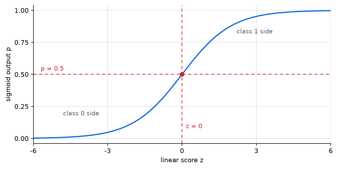
It becomes more intuitive on a coordinate plot. When the linear score \(z\) moves from negative to positive, the sigmoid output moves smoothly from near 0 to near 1, and it meets p = 0.5 at z = 0.
This flow can be drawn simply as follows.
flowchart TD
  A["features x"]
  B["linear score z"]
  C["sigmoid"]
  D["0-1 score"]
  E["class decision"]

  A --> B --> C --> D --> E
The key point is that logistic regression does not throw away the line. It keeps the linear calculation and adds one more transformation layer for interpretation.
What Is The Same And What Is Different Between Linear Regression And Logistic Regression?
The two models resemble each other because both use a linear combination. But the meaning of the output is different.
| Item | Linear regression | Logistic regression |
|---|---|---|
| Main problem type | regression | classification |
| Internal calculation | linear combination | linear combination |
| Final output | continuous value | 0-1 score and class decision |
| Introductory interpretation | predict points, minutes, money | estimate which class is more likely |
So logistic regression is not a model with a completely different starting point. It is a model that reinterprets the same linear structure for classification.
What Does predict_proba Show?
One of the important outputs in the scikit-learn logistic regression documentation is predict_proba. Readers often treat it immediately like the final answer, but in practice it is the information of one stage earlier.
For example, if the value is 0.82, it usually means the model considers the positive class fairly likely. But whether the final class is written as 0 or 1 is determined by the threshold.
In other words:
predict_proba: the degree of possibilitypredict: the final classification decision
If this distinction is missed, it becomes easy to confuse a score with a decision.
It becomes clearer in a tiny example.
| User | Class 1 score read through predict_proba | Decision under threshold 0.5 |
|---|---|---|
| A | 0.18 | class 0 |
| B | 0.49 | class 0 |
| C | 0.51 | class 1 |
| D | 0.87 | class 1 |
The important rows in this table are B and C. The difference in score is not large, but once threshold 0.5 is used, the final class changes. The score space created by the model is continuous, but the service decision can split discontinuously on top of it.
Why Is A Threshold Needed?
Logistic regression is often introduced first with the rule that it decides the class using 0.5.
- if the probability-like value is
>= 0.5, choose class 1 - if the probability-like value is
< 0.5, choose class 0
But this criterion is not a law of nature. It is a chosen policy.
In fraud detection, for example, the cost of missing a fraud can be high, so a service may want to catch cases more aggressively. In another service, blocking normal users too often may be unacceptable, so the threshold can be set more conservatively.
That means logistic regression produces a probability-like score, and the service decides where to draw the line on top of that score.
This point connects directly with the evaluation metrics of P4-6, the baseline of P4-8, and the tuning discussion of P4-9.
Consider one more small example.
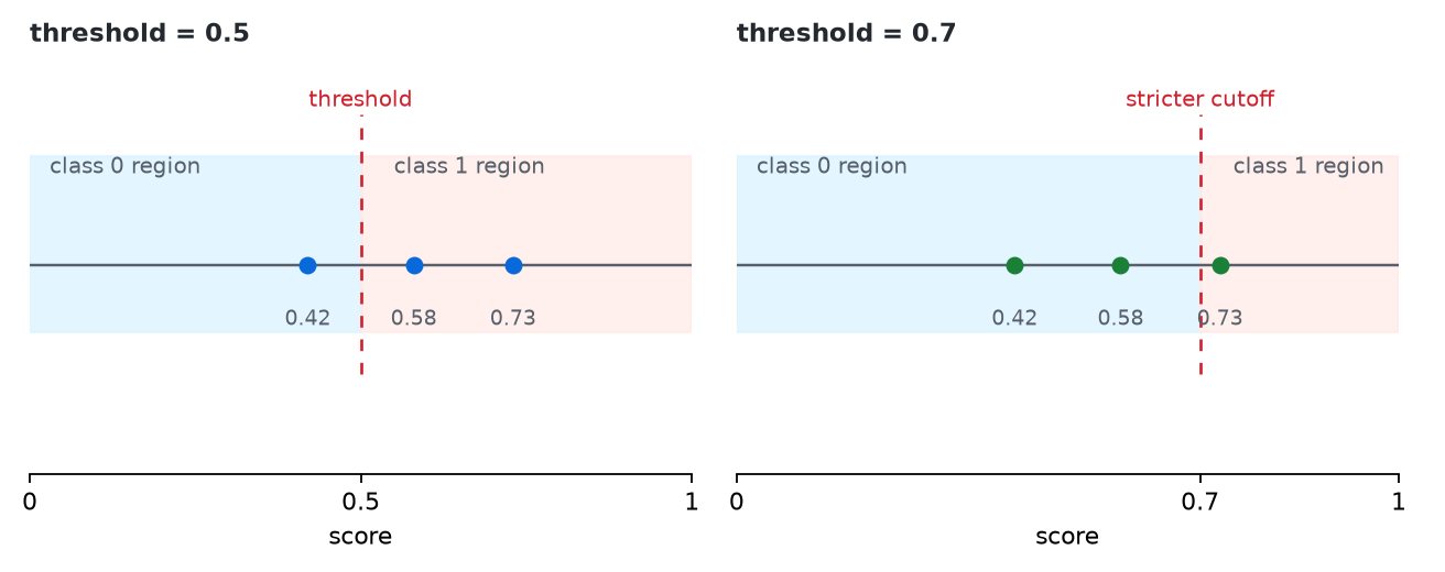
| Customer | Churn score | threshold = 0.5 | threshold = 0.7 |
|---|---|---|---|
| E | 0.42 | keep | keep |
| F | 0.58 | alert | keep |
| G | 0.73 | alert | alert |
Even with the same score, service behavior changes when the threshold changes. This is why logistic regression should be read with model score and operating policy separated. Cases near the boundary are first signals to raise review priority. Changing the threshold alone is not a complete explanation of the cause.
The same comparison frame should be kept here too. Thresholds must be compared over the same baseline, the same score range, and the same representative failure cases so that what changed because of policy and what remains because of weak representation do not get mixed together.
When this point is rewritten as project notes, it becomes even clearer. If logistic regression is used as the first comparison model, the team should not leave only the score table. It should also record which score range becomes a review target, which examples change behavior when the threshold changes, and what actually improved compared with the baseline.
| Record to keep together | Why it is needed |
|---|---|
| score comparison between the baseline and logistic regression | to see what really improved beyond a simple rule |
| examples of behavior changes by threshold | to record how service policy changes even with the same score |
| review score range | to reread near-boundary cases as human review candidates |
| next adjustment question | to decide whether to change the threshold, add features, or compare another candidate model |
This record keeps statements like the score improved, the threshold changed, and the number of alerts increased from being mixed together.
If the scene the same score leads to different final behavior depending on where the policy line is drawn is compressed onto one score axis, it can be read as follows.
When Is Logistic Regression A Good First Candidate?
Logistic regression is often the first comparison model for a classification problem, but the reason is not that it is simply famous. It is because it is a linear classification model that makes it comparatively easy to separate score and policy.
| Current problem state | Why raise logistic regression first | What to check first |
|---|---|---|
| the goal is binary classification | because it is easy to read both a 0-1 score and a final class together | whether the output is really a categorical decision |
| an explainable first classification model is needed | because the linear score, coefficients, and threshold can be explained relatively directly | whether a linear boundary is sufficient |
| a score model slightly stronger than the baseline is needed | because actual improvement beyond a majority-class rule is easy to compare | what changed inside the confusion matrix |
| a review score range should be left for humans | because predict_proba and threshold can be separated to define review targets | whether near-boundary cases are being recorded separately |
| service policy must be separated from model output | because the structure that the model makes the score and policy decides behavior stays visible | whether threshold change and model improvement are being mixed |
The key point of this table is to use logistic regression as both a comparison model that goes beyond a first classification baseline and a training model for reading score and policy separately.
Supplementary Reading Points
Academic Background And History
At this point, a natural question appears: why did a separate model like this need to exist? Because of the name, logistic regression can look like a simple variation of linear regression, but in practice it is closer to a model that extends a linear model that explained continuous values into a way of reading binary outcomes.
- Linear regression is strong at explaining continuous values.
- But if it is used as it is for a problem that chooses one of two outcomes such as success or failure, values below 0 or above 1 can appear, so it is hard to read them like probabilities.
- So statistics organized a reading method that keeps the linear formula but interprets its output inside the 0-1 range.
In that sense, the historical meaning of logistic regression is closer to re-reading a linear calculation for classification problems than to throwing away the line.
From this angle, the sequence between linear regression and logistic regression also becomes clearer.
- linear regression: the most basic linear model that explains continuous values
- logistic regression: a model that keeps the linear way of thinking but interprets the output for binary classification
In modern machine-learning contexts, this model is usually introduced as a linear model for classification. It is better not to memorize the full history, but to keep the following one sentence.
If linear regression was a representative linear model for explaining continuous values, logistic regression was the model that extended that same linear way of thinking toward binary classification and probability interpretation.
Where Do The Main Discussion Points Arise?
After seeing the operating idea and a few examples, the next question becomes how far should this model be trusted, and from where should the reader become careful? Logistic regression is often used as an introductory model, and it is also known as comparatively interpretable. But in practice it is also a model that looks easy to explain, so it is easy to oversimplify and misunderstand.
1. Are Score And Decision The Same Thing?
The most common misunderstanding is to treat the model output and the service action as though they were the same thing.
- The model usually emits a score close to
how likely is class 1? - The service decides actions such as
block,warn,review, orpasson top of that score
So the first discussion point around logistic regression is how far does the model speak, and where does service policy begin to intervene?
Logistic regression creates material for judgment, but it does not automatically determine the final behavior rule.
When rewritten in the form of operating notes, it can be recorded like this.
| Record item | Example |
|---|---|
| score | 0.58 |
| current threshold | 0.50 |
| current action | warn |
| whether review is needed | review because it is near the boundary |
| next question | if threshold rises above 0.60, how much does FN increase? |
2. Until When Is A Probability-Like Value Really A Probability?
Even if the output is 0.82, that does not automatically mean it perfectly represents the true real-world probability. Depending on data distribution, learning procedure, and calibration state, a score that looks like a probability and the actual observed frequency can differ.
The discussion point here is simple.
- Is this value closer to
a ranking score? - Or is it safe to read it as
a real-world probability?
This difference matters in practice. If the task is customer prioritization, the ranking may matter more. If the scene is something sensitive like medical risk guidance, calibration can matter much more.
The output of logistic regression is a score that can be read like a probability, but it does not always mean a perfectly calibrated real-world probability.
3. Is A Coefficient An Explanation Or A Cause?
One reason logistic regression is used widely is that its coefficients are comparatively readable. But being readable and knowing the cause are different things.
- The sign of a coefficient can show which direction pushes the score
- The size of a coefficient can provide a clue for relative influence inside the model
- But that does not by itself prove a direct real-world cause
This discussion point matters especially in social data, medical data, and user-behavior data. If correlation and causation are mixed together, the explanation may look easy while the conclusion becomes risky.
4. Is Logistic Regression Good Because It Is Simple, Or Weak Because It Is Simple?
Logistic regression is a linear model. That simplicity is both a strength and a limit.
- Strength: it is fast, works well as a baseline, and is comparatively easy to interpret
- Limit: when the relation between input and result is highly complex or nonlinear, its expressive power may be weak
That is why practice often leads to a question like this.
- Should the reader start with logistic regression and set the first reference line?
- Or should the reader move to a more complex model from the beginning?
This book takes the first route as the default. Logistic regression matters not because it is the best model, but because it is a good model for first understanding the structure of classification problems.
5. Why Is Threshold 0.5 Common, Yet Not An Absolute Criterion?
0.5 is only a common default. In real services, a different threshold can be more appropriate depending on cost structure, class imbalance, and policy goals.
- a service that must not miss spam
- a service that must not wrongly block normal users
- a service that must catch risk signals broadly and early
can all use different thresholds even on top of the same logistic regression output.
So one important discussion point around logistic regression is that a good score and a good action rule are not always the same thing.
Cases And Examples
Before reading the cases, the common comparison frame of this Section can be arranged as follows.
| Scene | Easy rule a person may use first | Limit of that rule | What logistic regression changes | Result to check |
|---|---|---|---|---|
| churn prediction | choose risky customers by intuition | the same customer can be judged differently by different people | keep a probability-like score and a threshold together | review targets and automatic actions can be separated |
| spam classification | block suspicious mail aggressively | FP and FN costs are easily mixed into one rough rule | read score and policy criterion separately | different service thresholds become explainable |
| medical risk classification | warn broadly when it looks risky | hard to handle miss cost and over-warning cost together | even the same score can be read with a more sensitive threshold | the need for criteria beyond accuracy becomes visible |
| loan / fraud detection | approve or block from one or two rules | easy to miss domain-specific cost differences | place different operating policies on top of the same model | model score and action policy stay separable |
Case 1. Why Does Logistic Regression Fit Churn Prediction Well As A First Model?
Logistic regression is often used like a baseline in churn prediction.
- the output value is
the likelihood of churn - the service decision is
from which score should a retention campaign begin?
Suppose a subscription service first looks only at the following three features.
| Customer | Login days in the last 30 days | Payments in the last 30 days | Complaint inquiry | Class 1 score | Action under 0.5 |
|---|---|---|---|---|---|
| A | 26 | 4 | none | 0.18 | keep normally |
| B | 9 | 1 | yes | 0.61 | retention campaign |
| C | 4 | 0 | yes | 0.84 | priority review plus strong retention |
The first thing to hold onto in this table is that input features do not go straight to action. The model creates a score first, and the service then divides actions such as keep normally, campaign, and human review on top of that score.
The reason logistic regression is often considered first here is usually threefold. A first reference line can be set quickly, the direction in which features push the score is comparatively readable, and several operating scenarios can be compared immediately by changing the threshold.
flowchart TD
  A["customer features"]
  B["linear score"]
  C["sigmoid"]
  D["class 1 score"]
  E["threshold policy"]
  F["campaign or review"]

  A --> B --> C --> D --> E --> F
In this scene, threshold policy matters more than the model name itself. Whether a customer like B at 0.61 becomes an automatic campaign target, or only customers like C above 0.80 receive stronger intervention, depends on cost structure. Even with the same score table, where automatic action starts is an operating decision outside the model.
Case 2. Why Is Spam Filtering Not Finished By The Probability Alone?
Imagine an email has a spam score of 0.49. Under threshold 0.5, it remains in the normal inbox. But this does not mean the message is certainly safe. It only means it falls on the class 0 side under the current threshold.
The service may still:
- surface it to a manual moderation queue,
- apply a softer warning,
- or compare it with representative false-negative cases.
This case shows why probability-like output and final behavior should not be read as the same sentence.
Case 3. Medical Risk Classification
In medicine, the cost of missing a positive-risk case can be very large. In that case, the service may need a lower threshold than 0.5 so that warnings are issued more sensitively.
For example, in an outpatient triage stage, the table may be read like this.
| Patient | Example signals the model saw | Class 1 score | Under 0.5 | Under 0.3 |
|---|---|---|---|---|
| P1 | younger age, main indicators stable | 0.11 | general guidance | general guidance |
| P2 | raised blood pressure, family history | 0.34 | general guidance | recommend extra test |
| P3 | several major indicators abnormal | 0.79 | recommend extra test | recommend extra test |
The key case here is P2. 0.34 may look low under a 0.5 rule, but in an environment where the cost of missing risk is high, recommending another test first may be safer.
In this kind of scene, plain accuracy alone is not enough. A viewpoint closer to sensitivity can matter more, so logistic regression is often used first as a score model, while the actual operation is designed separately together with medical criteria.
Case 4. The Difference Between Loan Review And Fraud Detection
In loan review, both false approval and false rejection are costly. In fraud detection, blocking normal users is costly too, but missing real fraud can be even more expensive.
Both tasks look like binary classification, but their operating perspectives differ.
- loan review: explainability and policy consistency can matter more
- fraud detection: fast warning and higher recall can matter more
| Scene | How a score of 0.62 may be read |
|---|---|
| loan review | it may be sent to additional document review or reviewer inspection rather than being rejected immediately |
| fraud detection | the system may react faster by temporarily holding payment or requiring extra authentication |
So even if the scores look similar, the same logistic-regression output can lead to different actions when the type of mistake the service can tolerate is different.
For that reason, the same logistic regression can survive as a long-lived baseline in some fields, while in other fields it is used mainly as a starting point before more complex models.
Logistic regression creates the score, and the service separately decides how to turn that score into action.
Practice And Example
Python Example: A Small Logistic Regression
The example below is a very small binary-classification practice that predicts whether a student passed from study_hours.
- problem situation: assume passing becomes more likely as study time increases
- input: study hours
- label: pass (
1) or fail (0) - concepts to check:
- the linear score is read as a 0-1 value after sigmoid
predict_probaandpredictare not the same stage- the sign of the coefficient shows which direction raises the chance
| Input bundle | Meaning |
|---|---|
study_hours | one-dimensional input with only one feature |
passed | pass / fail labels |
[[3], [5], [7]] | samples to inspect before the boundary, near the boundary, and after the boundary |
| Student | Study hours | Actual result |
|---|---|---|
| S1 | 1 | fail |
| S2 | 2 | fail |
| S3 | 3 | fail |
| S4 | 4 | fail |
| S5 | 5 | pass |
| S6 | 6 | pass |
| S7 | 7 | pass |
| S8 | 8 | pass |
Values to change:
- Replace
[[3], [5], [7]]with a denser set such as[[4], [5], [6]]to inspect score changes near the boundary. - Change one near-boundary label inside
passedto see whether the coefficient and intercept move together.
An example output is as follows.
This output can be read as follows.
- Because the coefficient is positive, more study time pushes the score toward the pass class.
- At
x=3, the value read like the class 1 probability is low, so the sample is classified on the fail side. - At
x=5, the class changes while passing near the 0.5 region. - At
x=7, the model sees the pass side as more likely.
The important point is that if a value such as 0.548 appears, it should not be read as an absolute fact. It should be read as the current model, after seeing this data, considers that class more likely.
Python Example: Reading predict_proba And predict Separately
The example below shows that logistic regression creates a score first and then turns it into a class through a threshold.
Values to change:
- Add values such as
0.48,0.50, and0.52toscoresto see how close scores become different class decisions near 0.5. - Change the cutoff in
pred_05to0.6to make the difference between score and decision more visible.
An example output is as follows.
This output shows that 0.49 and 0.51 are close as scores, but once the threshold is applied they end up on different sides of the final class decision.
Python Example: Reading Threshold Difference Together
Now, look directly at how the final behavior changes when the threshold changes, even if the score is the same.
- problem situation: assume the model has already produced churn scores
- input: computed class 1 scores
- expected output: how the decision changes under thresholds 0.5 and 0.7
- concept to check:
- the score may stay the same while the policy criterion changes the class decision
- the model output and the service action should be read separately
Values to change:
- Add
0.49,0.50, and0.51toscoresto see how the decision splits at the 0.5 boundary. - Change the cutoff in
pred_07to0.6or0.8to compare policy-only changes over the same score table.
An example output is as follows.
This output again shows that the model creates the score, but the operating rule decides how that score becomes behavior.
Change One More Value: How Does Interpretation Shake If One Near-Boundary Label Changes?
Now change the near-boundary case study_hours = 4 from fail (0) to pass (1) in the training data.
Values to change:
- Change the label at
study_hours = 3orstudy_hours = 5to see how score movement differs by boundary location. - Expand
predict_proba([[4]])to[[3]], [[4]], [[5]]to compare how the change spreads around the boundary.
An example output is as follows.
What Stayed The Same And What Changed?
- What stayed the same: the overall direction still says that more study time tends to raise the score toward the pass side.
- What changed: once one near-boundary label changed, the class 1 score at
x=4moved sharply from0.327to0.579. - Judgment to leave first: the score of logistic regression is not a probability discovered from nature. It is an interpretation produced by the current data boundary.
This exercise makes logistic regression readable again not merely as a model that prints scores, but as a classification rule that is sensitive to near-boundary examples. What matters is not trusting one score by itself, but reading how a change in one example shakes score interpretation and threshold judgment. Repeating the same example with one changed value makes it more visible that there is always one more layer between model output and service action: data interpretation.
| Common record language | What to record immediately from this exercise |
|---|---|
| structure observed | even one changed near-boundary label strongly changed the interpretation of the class 1 score for the same input |
| interpretation boundary | this score change alone does not prove that the real-world probability suddenly changed; the sample and the data boundary still need to be read together |
| next question | if more near-boundary cases are collected, does the score become less unstable, and what changes once threshold policy is added? |
| Signal seen first | What that signal means | Immediate next action |
|---|---|---|
| Many scores are near 0.5 and the judgment flips often when the threshold changes | The operating boundary is making a bigger difference than the score itself | Collect more near-boundary cases and review the threshold against FP and FN costs |
| Scores are high, but the observed frequency and felt risk still seem misaligned | Reading ranking and probability as the same thing may be risky | Recheck whether calibration is needed or whether the score should remain only a ranking signal |
Checklist
- Did you first confirm that the current task is binary classification?
- Can you explain logistic regression as a linear model that produces outputs that can be read like probabilities in a classification problem?
- Do you understand that the internal calculation is still a linear combination, but the final interpretation changes into a 0-1 range through sigmoid?
- Are you avoiding reading
predict_probaand finalpredictas the same thing? - Can you explain threshold change separately from improvement of the model itself?
- When coefficient interpretation, sigmoid, and probability-like output feel tangled together, can you explain again that logistic regression is a model with one more interpretation layer after the linear combination?
Sources And References
- scikit-learn,
1.1.11. Logistic regression, scikit-learn User Guide, checked on 2026-07-26. https://scikit-learn.org/stable/modules/linear_model.html#logistic-regression - scikit-learn,
LogisticRegression, scikit-learn API Reference, checked on 2026-07-26. https://scikit-learn.org/stable/modules/generated/sklearn.linear_model.LogisticRegression.html