P4-11.2 Decision Boundary
Section ID:
P4-11.2Version:v2026.07.31
In P4-11.1, logistic regression was read as a linear model that creates scores that can be read like probabilities. Now the question changes by one step.
Why does that score divide some inputs into class 0 and others into class 1?
To answer that, it is not enough to ask only what is the probability? The reader also has to see up to where is it read as class 0, and from where is it read as class 1? The perspective that reads that criterion inside the input space is the decision boundary.
So the phrase where does the model draw a line in the input space? is closer to a result than the deepest idea. The more essential question is the following.
By what rule does the model read inputs as two different sides?
If P4-11.1 was the Section of reading the output, P4-11.2 is the Section of looking back at the input.
A decision boundary is the criterion line or criterion surface that separates class 0 and class 1.
This Section does not repeat the basic definition of logistic regression at length. The core intuition, a linear classifier that makes a score that can be read like a probability, reconnects through P4-11.1 and the glossary entries for logistic regression and decision boundary. Here the focus stays on how that score divides the input space.
After reading the decision boundary, the next questions remain: why is probability transformed and read in this way, why do log-odds and MLE follow in the explanation of learning, and how does this intuition widen to multiclass settings and model comparison. That recovery continues in the supplementary learning of P4-11.3, P4-11.4, and P4-11.5.
Questions Closed By Decision Boundary
This Section answers the following questions.
- What is a decision boundary?
- How does the boundary look in a one-dimensional input?
- Why does it look like a line in a two-dimensional input?
- How do coefficients relate to the direction of the boundary?
- How can the boundary change when the threshold changes?
This Section first closes the decision boundary as the criterion that divides the input space, and focuses on holding onto how the threshold that appeared in output scores is read as a boundary in the input space.
At the same time, the broader questions that should be revisited later are also clear. The hyperplane intuition reconnects again in P4-1.2, and kernel methods and nonlinear boundaries return in P4-13.1 and P4-13.2. Settings and computation costs such as C, gamma, and threshold adjustment reconnect again in P4-9.1 and P4-9.2, and multiclass expansion continues in P4-11.4.
Judgments To Keep From Decision Boundary
- You can explain a decision boundary not as
an output scorebut asa criterion that divides the input space. - You can understand that in one dimension the boundary looks like
one point, and in two dimensions it usually looks likeone line. - You can explain that the coefficients of logistic regression participate in changing the direction of the boundary.
- You can explain that when the threshold changes, the boundary itself can move too.
- You can connect the probability-output view of 11.1 and the boundary view of 11.2 as two descriptions of the same model.
Learning Background
Why Read The Decision Boundary Separately?
In 11.1, the reader saw scores such as 0.58 and 0.73. But in practice and in learning, the following questions often matter more.
- Why did one input become class 0?
- Why did another input become class 1?
- Where is the criterion that separates the two classes?
Those questions cannot be answered sufficiently from an output table alone. The output table shows the result, but not enough of why that result appeared.
This is why the decision boundary is needed.
- to explain why an input became class 0
- to explain why an input became class 1
- to say where the criterion that separates the two classes lies
- to identify near-boundary cases that should be treated separately
So the decision boundary is not merely a visualization device. It is an interpretation tool for reading why classification happened.
The perspective that appears when we need to ask where did the model divide the space into two sides? is the decision boundary.
It should also be read together with the following four items.
| What to read together | Why it is needed |
|---|---|
| baseline classification result | because we still need to know whether the linear boundary is actually better than a simple rule |
| threshold position | because the criterion that changes the class must be visible even with the same score |
| problem cells in the confusion matrix | because we need to see what kind of misclassification the boundary is creating |
| representative near-boundary examples | because we need to explain why ambiguous inputs crossed to the opposite side |
So this is not a Section about drawing a line prettily. It is a Section about reading together what improved compared with what, where the class changes, and what type of error appears as a result.
If one more point is added, the decision boundary becomes even more directly connected to operational interpretation. Near-boundary cases are not just ambiguous points. They are cases that should be left first as priority review targets. In that sense, the decision boundary can also be read as a comparison frame for deciding which inputs should be checked by a human again. The fact that a case lies near the boundary shows a change signal and review priority. It does not automatically complete the causal explanation of why the case crossed.
The same comparison frame should be kept here too. The same baseline, the same score ranges, and the same representative failure cases should be used before and after the boundary so that model score change, threshold policy change, and lack of feature representation are not mixed together too easily.
| What to keep when reading the boundary | Why it is needed |
|---|---|
| IDs of near-boundary examples | to find review targets again |
| changed classifications relative to the baseline | to see which cases were newly separated compared with a simple rule |
| cases that moved after a threshold change | to see which inputs crossed because of a policy change |
| next review question | to decide whether to add features or adjust the threshold |
If this record is kept, the boundary moved, warnings increased, and newly split cases appeared can be reread inside one comparison frame instead of being read separately.
A Decision Boundary Is Where Classification Judgment Flips
A classification model usually computes an internal score and divides classes based on that score. The decision boundary is the place where that score becomes equal to the criterion value.
If 11.1 was the Section of reading threshold on the output-score axis, here the focus is only on what kind of boundary that threshold becomes in the input space.
If logistic regression is simplified at an introductory level, it can be imagined as follows.
If this linear score \(z\) is passed through sigmoid, a value between 0 and 1 appears. When threshold 0.5 is used, the place where the sigmoid output becomes 0.5 becomes the class boundary.
Sigmoid output 0.5 corresponds to the linear score \(z = 0\). So the decision boundary of logistic regression can usually be understood as the place where the linear score becomes 0.
The decision boundary is the place where the probability becomes ambiguous and the place where the class splits.
In One Dimension, The Boundary Looks Like One Point
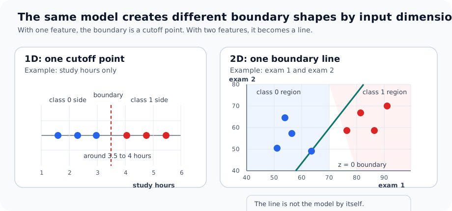
If there is only one input, the boundary appears not as a line but as one point.
Suppose the input is just study_hours. The model can separate fail and pass using some time value as the criterion.
| Study hours | Class 1 score | Prediction |
|---|---|---|
| 3 | 0.17 | fail |
| 4 | 0.31 | fail |
| 5 | 0.55 | pass |
| 6 | 0.76 | pass |
In this case, the boundary can be read as lying somewhere between 4 and 5 hours. So a one-dimensional decision boundary is close to one cutoff point.
If the cutoff point for one variable and the boundary line for two variables are compared in the same figure, it can be read as follows.
The idea can be drawn simply as follows.
flowchart TD
  A["study_hours increases"]

  subgraph L["class 0 side"]
    direction TB
    L1["3h<br/>score 0.17"]
    L2["4h<br/>score 0.31"]
  end

  B["boundary<br/>score 0.50"]

  subgraph R["class 1 side"]
    direction TB
    R1["5h<br/>score 0.55"]
    R2["6h<br/>score 0.76"]
  end

  A --> L
  L --> B --> R
The key in this diagram is that as the input value increases, the score rises, and around the score 0.50 boundary point the model splits the axis into the class 0 side and the class 1 side. So in one dimension, the boundary is read not as a complicated plane or region, but as one point on the axis.
This becomes especially important when threshold is inspected. What looked like a score table in 11.1 starts to reappear in 11.2 as a boundary point on the input axis.
In Two Dimensions, The Boundary Looks Like A Line
Now suppose there are two inputs, such as exam_1 and exam_2, and the task is to classify pass or fail. Then the input space is easier to imagine as a plane rather than as a single table.
- one axis is
exam_1 - the other axis is
exam_2 - each student becomes one point on that plane
In this setting, logistic regression tries to find the criterion line that separates those points into two sides. So in two dimensions the decision boundary usually appears like a line.
flowchart TD
  A["input point (exam_1, exam_2)"]
  A --> B["linear score z"]
  B --> C{"z vs 0"}
  C -->|z < 0| D["class 0 side"]
  C -->|z > 0| E["class 1 side"]
  C -->|z = 0| F["boundary"]
This diagram shows the decision boundary of logistic regression as the trace left in the input space by the rule that compares the score \(z\) with zero. What matters is not drawing the line itself, but reading that the class splits depending on which sign the linear score has.
When one more input dimension is added, the boundary changes from one point to one line.
The important point here is not there is a line first and then the class splits, but because the rule compares z with 0, a boundary line appears as a result on the plane.
The most direct answers to the following three questions in two dimensions are the same.
- Why did one input become class 0?
Because its z is smaller than 0 - Why did one input become class 1?
Because its z is larger than 0 - Where is the criterion between the two classes?
The set of all points where z = 0
So the decision boundary should be read not as a simple picture, but as the trace left on the plane by the classification rule.
How Do Coefficients Relate To The Direction Of The Boundary?
The coefficients of logistic regression are not used only to compute the score. When viewed in the input space, they also influence the direction in which the boundary is placed.
If there are two features,
then the relative size and sign of \(w_1\) and \(w_2\) change the slope and direction of the boundary line.
The following intuition is more important than a formal derivation.
- If the coefficient of one feature becomes larger, the influence of that axis can become stronger.
- If the combination of the two coefficients changes, the tilt of the class-separating boundary changes too.
- The intercept shifts the boundary in parallel.
So in 11.1 the coefficients were numbers that make a score, while in 11.2 they also become numbers that define a boundary.
The Boundary Can Move If The Threshold Changes
In 11.1, the reader saw that the final behavior changes when the threshold changes. In 11.2 that statement has to be reread from the spatial perspective.
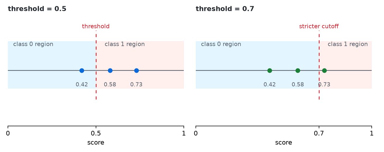
The boundary under threshold 0.5 and the boundary under threshold 0.7 do not need to sit at the same place. The reason is simple.
- threshold 0.5: choose class 1 from the place where the score crosses this level
- threshold 0.7: require a higher score before class 1 is chosen
So when the threshold rises, the region classified as class 1 can shrink, and the boundary can move in a more conservative direction.
The coefficients of the model create the direction of the boundary, and the threshold can readjust where that boundary is applied.
If the same score arrangement is kept and only the threshold changes, the cutoff shift on the score axis becomes a smaller class 1 region in the input space. That coordinate-style comparison can be read as follows.
This movement can be drawn conceptually as follows.
flowchart TD
  A["same score axis"]

  subgraph L["threshold 0.5"]
    direction TB
    L1["boundary earlier"]
    L2["class 1 region wider"]
  end

  subgraph R["threshold 0.7"]
    direction TB
    R1["boundary moves right"]
    R2["class 1 region smaller"]
  end

  A --> L
  A --> R
  L --> R
The key is that even without retraining the model, a stricter threshold pushes the effective boundary to the right on the same score axis and reads a smaller class 1 region. So a boundary shift should be read as a policy change that changes which cases cross the line, not as a complete causal explanation of the features.
The following three lines should be kept together in decision-boundary notes.
- Near-boundary cases are signals to raise review priority, not automatic confirmation.
- If the threshold changes, the same input can move to a different action.
- A boundary shift can be observed, but the shift itself does not finish the causal explanation.
When Is The Decision-Boundary Perspective Especially Important?
The decision boundary is not just a visualization scene. It becomes especially important when the reader must ask why did this input cross into the other class?
| What the reader wants to inspect now | Why the decision-boundary perspective is needed | What to check together |
|---|---|---|
| ambiguous cases near the boundary | because the score alone does not explain well why they split | threshold and the review zone |
| repeated misclassification of one type | because the reader must see how the boundary is tilted | the problem cells of the confusion matrix |
| deciding whether to change the threshold | because the effect of the policy change must be read in the input space | changes in cases before and after the threshold |
| suspecting that more features are needed | because the current boundary may be too simple | cases newly separated compared with the baseline |
| selecting human-review targets | because near-boundary cases define review priority | case IDs and score ranges |
The point of this table is not to admire the picture of the boundary, but to track where the classification rule really splits and what it misses.
Background for Reading Decision Boundaries as Spatial Separation Criteria
At first glance, the phrase decision boundary can look like a visualization term. But the core is not the picture. It is the perspective of reading where a classification judgment flips.
If the early regression tradition was closer to how well is the value explained, classification changes the question to which class does it go to. At that point the model starts to be read not only as a function that outputs scores, but also as a device that divides the input space into two sides.
Explanations around Fisher's discriminant tradition, the Bayes classifier, and LDA/QDA also ultimately connect to the language of where does the class change. So the decision boundary is more accurate when understood not as the technique of drawing lines in space, but as a way to express the criterion at which a classification judgment flips.
Logistic regression can be summarized from that perspective as follows.
- 11.1's perspective: logistic regression creates scores that can be read like probabilities
- 11.2's perspective: logistic regression draws a boundary in the input space and divides classes
These two perspectives are not different models. They are two ways of reading the same model.
The reason the decision-boundary perspective matters in modern machine learning is also clear. Models that appear later, such as SVMs, decision trees, and neural networks, can all be reread through the question how does the model divide the input space?
So the historical meaning of the decision boundary can be summarized at the introductory level as follows.
Classification is a problem of calculating scores, but at the same time it is also a problem of how to divide the input space.
If this sentence is clear, the reader can understand more directly why other classification algorithms follow logistic regression.
Cases And Examples
Before the cases, the common comparison frame of this Section can be organized as follows.
| Scene | Easy rule a person might use first | Limit of that rule | What the decision-boundary perspective changes | Result to check |
|---|---|---|---|---|
| exam-pass prediction | use one cutoff on one score | weak when several features act together | read it as a combined criterion | the boundary becomes a line or plane rather than one point |
| customer churn | judge risk from one variable | misses combined patterns | check whether a combination of features creates a risk region | explain which combinations lie beyond the boundary |
| medical risk | judge risk from one number | misses ambiguous combinations | separate near-boundary cases for review | identify review-priority targets |
| loan / spam | explain approval or blocking with one simple rule | misses mixed features and the limit of a linear boundary | inspect which combinations the boundary separates | read both the strength and the limit of a linear boundary |
flowchart TD
  A["many features"]
  B["single-rule reading"]
  C["mixed patterns"]
  D["boundary view<br/>which side of z = 0"]
  E["near-boundary review"]
  F["why it crossed"]

  A --> B --> C --> D
  D --> E
  D --> F
Case 1. Pass Prediction
If there is only one score, one cutoff point becomes the boundary. But if there are two subjects, a tradeoff can appear, such as high math score but low English score. Then a boundary line that reads two scores together fits better than a criterion on only one subject.
The same scene can be read through a small table as follows.
| Student | Math score | English score | Boundary interpretation |
|---|---|---|---|
| A | 92 | 38 | one subject is high, but the student may remain near the boundary because the other is low |
| B | 71 | 68 | both scores are together above the middle, so the student can cross toward the pass side more easily |
| C | 45 | 44 | both scores are low, so the student is likely to remain on the fail side |
The key in this table is that a single rule such as is math above 90? does not explain the difference between A and B well enough. The decision-boundary perspective makes the reader inspect on which side of the region the combination of the two scores lies.
This case matters because readers easily keep understanding classification as if it were only one passing line on one score. The decision-boundary perspective shows that when several features work together, the criterion also changes into a combination.
Case 2. Customer Churn Prediction
When the inputs become several variables such as recent login days, payment frequency, and customer-service inquiry count, it becomes hard to explain churn from only one variable. The decision-boundary perspective helps the reader ask which combinations of several features enter the risky region?
For example, compare the following three customers.
| Customer | Login days in the last 30 days | Payments in the last 30 days | Inquiry count | Boundary interpretation |
|---|---|---|---|---|
| A | 22 | 3 | 0 | likely to remain in the retain region |
| B | 11 | 1 | 2 | easy to read as a near-boundary review target |
| C | 4 | 0 | 4 | easy to read as having crossed into the risky region |
B is the important case here. Login days alone are not extremely low, but if payment frequency falls and inquiries rise together, the sample can become a near-boundary case.
For example, even if logins have decreased a little, stable payments can still keep a customer on the retain side. But if lower logins and payment interruption appear together, the customer can cross into the risky region. So the boundary makes the reader inspect not one value, but the pattern of the combination.
Case 3. Medical Risk Classification
One measurement alone may look ambiguous, but if blood pressure, blood sugar, and age are read together, the risky region can become clearer. The decision boundary helps the reader imagine which combinations cross into the risk class.
A small version can be arranged as follows.
| Patient | Blood pressure | Blood sugar | Age | Boundary interpretation |
|---|---|---|---|---|
| P1 | normal | normal | 34 | far from the risky region |
| P2 | slightly high | near boundary value | 58 | can require additional review as a near-boundary case |
| P3 | high | high | 67 | easy to read as having crossed into the risky region |
P2 is the key in this scene. One value alone may still look ambiguous, but if several values are all close to the boundary at the same time, a real decision has to be more careful.
In this example, the patient near the boundary matters especially. A patient whose score is obviously high can be easier than a patient whose several values overlap ambiguously near the boundary. So the decision boundary helps not only with simple classification, but also with reading which cases are ambiguous.
Case 4. Loan Review
In loan review, features such as income, debt ratio, delinquency record, and employment duration can work together. The decision-boundary perspective is useful for explaining which applicants are in the approval region and which are in the rejection region.
A small example can be read as follows.
| Applicant | Income | Debt ratio | Delinquency record | Boundary interpretation |
|---|---|---|---|---|
| D1 | high | low | none | easy to read as being on the approval side |
| D2 | medium | high | none | may require extra-document review near the boundary |
| D3 | low | high | yes | easy to read as having crossed into the rejection side |
D2 is difficult to explain with a single rule. Income alone may not look too bad, but a high debt ratio can change where the boundary is read.
The important point is that there are applicants who cannot be explained well by one criterion alone. Income can be high while debt ratio is also high, and employment duration can be short while delinquency record is absent. This kind of combined judgment is hard to explain without the decision-boundary perspective.
Case 5. Separating Spam And Normal Mail
In email classification, word frequency, sender pattern, number of links, and subject expression can all work together. Then the boundary makes the reader ask which mails leave the normal-mail region and cross into the spam region?
A small table can be read as follows.
| Number of links | Suspicious sender | Subject expression | Boundary interpretation | |
|---|---|---|---|---|
| M1 | 0 | no | ordinary work subject | close to the normal region |
| M2 | 2 | no | exaggerated expression present | can require human review as a near-boundary case |
| M3 | 5 | yes | repeated exaggerated wording | easy to read as having crossed into the spam region |
M2 matters because there are many links alone does not close the explanation. Only when it is placed with the other features does it become clearer whether it is a near-boundary case.
This case shows both the strength and the limit of a linear boundary. A simple separation is fast and easy to explain, but real spam mixes many forms, so one straight line may not be enough.
Practice And Example
Python Example: Reading A Two-Dimensional Decision Boundary
This example is a very small binary-classification exercise that classifies whether a student passed using two exam scores, exam_1 and exam_2.
- problem situation: the assumption is that passing becomes more likely when both scores are high together
- input: scores from two subjects
- label: pass (1) / fail (0)
- concept to check:
- logistic regression computes one score using the two features together
- two coefficients and one intercept participate in the position and direction of the decision boundary
- even in the same input space, classes split on the two sides of the boundary
The inputs can be read as follows.
| Input bundle | Meaning |
|---|---|
X | two-dimensional input made of the two subject scores |
y | pass / fail labels |
samples | samples to inspect below the boundary, near the boundary, and above the boundary |
Values to change:
- Change
samplesmore densely to[48, 49],[50, 50], and[52, 51]to inspect score movement near the boundary. - Move one or two points in
Xto see whether the coefficients, intercept, and boundary interpretation move together.
An example output is as follows.
This output can be read as follows.
- Because both coefficients are positive, the score moves toward class 1 when the two subject scores rise together.
[42, 42]sits on the class 0 side of the boundary.[50, 50]is near the boundary, so the probability-like value also appears near 0.5.[62, 60]is far enough inside the class 1 side.
The point that decision score is close to 0 can be read as meaning that the sample is near the boundary. This connects exactly to the explanation in 11.1 that predict_proba becomes ambiguous when it is near 0.5.
The same content becomes clearer if it is reread as a table.
| Sample | Input | Decision score \(z\) | Relation to the boundary \(z = 0\) | Prediction |
|---|---|---|---|---|
| A | [42, 42] | -4.102 | lower than the boundary | class 0 |
| B | [50, 50] | 0.187 | just above the boundary | class 1 |
| C | [62, 60] | 12.979 | far above the boundary | class 1 |
In actual operation, this way of reading continues directly.
- Samples far from the boundary are easier to treat as automatic candidates.
- Samples very near the boundary are easier to separate as review targets.
- So the decision boundary is not just a picture. It also connects to an operating criterion for finding ambiguous cases.
Python Example: Confirm Threshold Change With A Small Script
This time, use class 1 scores that have already been calculated and check how the boundary interpretation changes when the threshold changes.
Problem situation:
- even with the same probability score, the final class judgment changes depending on where the threshold is placed
Input:
- class 1 scores of three samples,
proba_class_1
Expected output:
- classification result under threshold 0.5
- classification result under threshold 0.7
Concept to check:
- changing the threshold changes the size of the class regions
- the boundary is connected not only to a formula, but also to an operating rule
Values to change:
- Add
0.49,0.50, and0.51toproba_class_1to see how classes split at the 0.5 boundary. - Change the cutoff in
pred_07to0.6or0.8to compare how much the class 1 region changes over the same score array.
An example output is as follows.
This result shows that a point such as 0.62 can already look fairly positive from the model's perspective, but under a stricter threshold it can still remain outside the class 1 region.
Change One More Value: What Stays The Same And What Changes If The Threshold Becomes Even Higher?
Now keep the same score array and raise the threshold again to 0.9.
Values to change:
- Change
0.81to0.91to see which cases still remain automatic class 1 under a high threshold. - Change
pred_09to an0.85cutoff to compare how the review candidates change when the operating criterion is lowered slightly.
An example output is as follows.
What Stayed The Same And What Changed?
- What stayed the same: the relative order of the scores is unchanged.
0.81is still closest to class 1, and0.48is still the farthest. - What changed: once the threshold rose again, even
0.81, which used to look like an automatic candidate, no longer became class 1 automatically. - Judgment to leave first: the score itself and the final behavior are not the same stage. Not only near-boundary cases, but even cases that once looked certain can return to the review pool when the operating criterion changes.
This comparison makes a classification model readable as an operating-boundary adjustment device, not just as a probability calculator. What matters is not only making one score higher, but reading which cases move from automatic handling back to review when the threshold changes and which error costs move with them. Repeating the same score array while changing only the boundary trains the reader to separate model output from applied judgment.
| Common record language | What to record immediately from this exercise |
|---|---|
| structure observed | even with the same scores, raising the threshold shrank the class 1 region and returned an automatic case to review candidacy |
| interpretation boundary | a more conservative threshold is not automatically a better service policy, because the increased FN cost must be read together |
| next question | should the team first compare whether the reduced FP is really more important than the increased FN and review load? |
Supplementary Reading On Detailed Content
Where Do The Main Discussion Points Arise?
Even though the decision boundary can look simple as a picture, there are several places where readers often misunderstand it.
1. Is The Boundary A Wall?
No. The decision boundary is not a physical wall in the real world. It is a separating criterion drawn by the model for convenience. Samples near the boundary can cross into the other class with a small change.
2. Does Farther From The Boundary Always Mean More Certain?
In logistic regression, points farther from the boundary usually tilt the score more strongly toward one class. But that does not guarantee perfect certainty in the real world. Data quality and data distribution still matter.
3. Is A Linear Boundary Always Enough?
No. If the data are mixed in a curved shape, or if the class structure is very complex, one line may not be enough. That limitation is why more complex models appear later.
4. Does The Boundary Stay Fixed Even If The Data Change?
No. If the training data change, the coefficients and intercept can change, and then the position and direction of the boundary can change as well. So a decision boundary is closer to a learning result produced by the current data and model than to a line discovered from nature.
This point connects directly with why train/test split, sample bias, and dataset updates matter.
5. Why Should Near-Boundary Samples Be Treated Carefully?
Samples far from the boundary are usually classified more stably. Samples near the boundary can switch class with a small change.
Because of that, real services often attach policies such as the following.
- if the point is far from the boundary, handle it automatically
- if it is near the boundary, send it to human review
- gather near-boundary cases separately for quality inspection
So the decision boundary can be used not only to split classes, but also to find which cases are ambiguous and operationally risky.
6. Are A Good Boundary And A Good Service Always The Same Thing?
Not necessarily. A boundary may look clean from the model perspective but still be inappropriate from the service perspective. If the cost of misclassification differs across classes, the safest operating boundary may differ from the mathematically neatest one.
This point connects to the threshold of 11.1, the evaluation metrics in the early part of Part 4, and model selection later.
Checklist
- Are you looking not only at output scores but also at where the split occurs in the input space?
- Are you separating cases that crossed because of threshold change from cases that failed because the feature representation was too weak?
- Are you leaving near-boundary cases not as automatic confirmations but as review-priority signals?
- Can you explain that the decision boundary is not a picture decoration, but a way to read where the classification rule flips?
- Can you explain that coefficients and intercept shape the direction and position of the boundary, while threshold can move the applied criterion?
- Can you explain that near-boundary cases are important not because they automatically prove a cause, but because they become review-priority signals?
Sources And References
- Ronald A. Fisher,
The Use of Multiple Measurements in Taxonomic Problems, Annals of Eugenics, 1936, DOI: https://doi.org/10.1111/j.1469-1809.1936.tb02137.x, checked on 2026-07-26. - Benyamin Ghojogh, Mark Crowley,
Linear and Quadratic Discriminant Analysis: Tutorial, arXiv, 2019, https://arxiv.org/abs/1906.02590, checked on 2026-07-26. - scikit-learn,
1.1.11. Logistic regression, scikit-learn User Guide, checked on 2026-07-26. https://scikit-learn.org/stable/modules/linear_model.html#logistic-regression - scikit-learn,
LogisticRegression, scikit-learn API Reference, checked on 2026-07-26. https://scikit-learn.org/stable/modules/generated/sklearn.linear_model.LogisticRegression.html