P4-11.3 Supplementary Learning: How To Read Log-Odds And MLE For The First Time
Section ID:
P4-11.3Version:v2026.07.31
P4-11.1 introduced logistic regression as a linear classification model that creates scores that can be read like probabilities, and P4-11.2 reread those scores as a decision boundary inside the input space. At that point a natural next question remains.
Why is probability not handled directly as a linear formula, and why do terms such as log-odds and maximum likelihood estimation (MLE) appear?
This Section is a supplementary learning path that closes that question. Its center is the probability interpretation of logistic regression and the learning objective. Multinomial expansion and solver or regularization settings are separated into P4-11.4 and P4-11.5.
Questions Closed By Log-Odds And MLE
This Section answers the following questions.
- Why does log-odds appear?
- Why is logistic regression said to learn by maximum likelihood estimation (MLE)?
- How does log loss connect to MLE?
This Section first closes log-odds and MLE as the criteria that connect probability interpretation and learning objective, and focuses on holding onto why the same model is reread in this mathematical language.
At the same time, the broader questions that should be revisited later are also clear. Multinomial expansion continues in P4-11.4, and solver and regularization continue in P4-11.5.
Judgments To Keep From Log-Odds And MLE
- You can explain the relationship among probability, odds, and log-odds at an introductory level.
- You can explain that
z = 0,probability 0.5, andodds 1point to the same place. - You can explain that logistic regression is trained in the direction that gives high probability to the correct answer.
- You can read MLE and log loss as two expressions of the same training objective.
Learning Background
Logistic regression often begins with the explanation that sigmoid is attached so the output can be read as a value between 0 and 1. That is enough for first understanding, but a little later the reader encounters the following terms.
- logit or log-odds
- likelihood or log-likelihood
- MLE
- log loss
Readers often get stuck here because the language suddenly starts sounding like a mathematics textbook. But these names are not separate. They are different ways of reading the same question.
- Probability is bounded between 0 and 1, so it is hard to connect directly to a linear formula.
- That is why log-odds appears to connect probability to a linear score.
- Classification learning needs to ask
how much probability did the model assign to the correct answer? - That is why likelihood, MLE, and log loss appear together.
So the key point is not to memorize new algorithms. It is to understand why probability interpretation and learning objective appear together in the same chapter.
Log-Odds Appears Because Probability Is Hard to Handle Directly With a Linear Formula
As seen in P4-11.1, logistic regression creates a linear score \(z\) and then passes it through sigmoid to read it as a value between 0 and 1.
If this expression is read backward step by step, as if solving probability p back into z, the following flow appears.
If the logarithm is taken at the end, the following relationship appears.
On the left, \(\frac{p}{1-p}\) is the odds, and its logarithm is the log-odds or logit. This relationship matters for a simple reason.
- probability \(p\) is trapped between 0 and 1
- the linear score \(z\) can move freely across negative and positive values
- so a transformation such as log-odds is needed as a bridge between
a scale that is easy to handle linearlyanda scale that is easy to read like probability
So log-odds is not a needlessly difficult word. It is the bridge that connects probability to a linear formula.
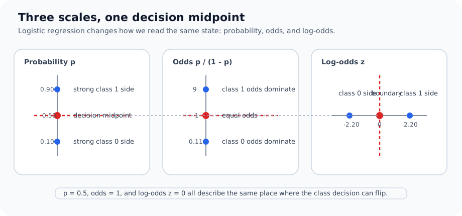
The intuition becomes clearer in a tiny table.
| Probability \(p\) | odds \(p / (1-p)\) | log-odds |
|---|---|---|
| 0.10 | 0.111 | -2.197 |
| 0.50 | 1.000 | 0.000 |
| 0.80 | 4.000 | 1.386 |
| 0.90 | 9.000 | 2.197 |
This table says the following.
- probability 0.5 corresponds to log-odds 0
- stronger confidence toward class 1 makes log-odds grow positive
- stronger confidence toward class 0 makes log-odds grow negative
That means the explanation in P4-11.2, the decision boundary is where the linear score \(z = 0\), can be reread again as saying that probability 0.5, odds 1, and log-odds 0 all point to the same place.
This correspondence is better held not as a table to memorize, but as reading the same state on different scales.
flowchart TD
  A["linear score z"]
  B["sigmoid"]
  C["probability p"]
  D["odds p / (1-p)"]
  E["log-odds = z"]

  A --> B --> C --> D --> E
Maximum Likelihood Estimation (MLE) Means Finding Parameters That Give High Probability To The Correct Answer
In linear regression, it feels natural to think in terms of reducing squared error. In classification, however, the correct answer is 0 or 1, so what matters more is not how close was the continuous value? but how much probability was assigned to the correct class?
That is why logistic regression is usually explained in terms of maximizing the likelihood, or more often the log-likelihood.
If the true label \(y_i\) of one binary-classification sample is 0 or 1, and the model's probability for class 1 is \(p_i\), the probability of one sample can be written in the following compact line.
This can look unfamiliar at first, but it only compresses the idea use \(p_i\) when the correct answer is 1, and use \(1-p_i\) when the correct answer is 0.
- if \(y_i = 1\), then \(p_i^{1}(1-p_i)^0 = p_i\)
- if \(y_i = 0\), then \(p_i^{0}(1-p_i)^1 = 1-p_i\)
For the whole dataset of \(n\) samples, the likelihood is gathered as a product.
Because products are hard to handle, the logarithm is usually applied to create a log-likelihood.
And in implementation this is often used not by maximizing the value, but by putting a minus sign in front and minimizing the negative log-likelihood.
This is the core shape of the log loss that appears often in binary logistic regression.
Read one line at a time, the meaning is the following.
- One sample is read by
the probability given to the correct answer. - The full dataset is read by
multiplying the probabilities of all samples. - A logarithm is taken so the product becomes a sum that is easier to handle.
- In implementation it is often easier to minimize, so a minus sign is added.
At an introductory level, the following one sentence is enough to hold first.
Maximum likelihood estimation is the method that finds parameters so the model explains the observed correct answers as plausibly as possible.
MLE Shows Why Accuracy Alone Cannot Explain Training
A common misunderstanding at the introductory stage is: if this is classification, can't we just count the number of correct predictions? Accuracy can matter in evaluation, but training must distinguish more delicate differences.
Suppose the true answer of a sample is 1.
- Model A gives probability 0.51, so it barely gets it right.
- Model B gives probability 0.99, so it gets it right much more confidently.
Accuracy reads both as simply correct. But learning should not treat them as identical. MLE is exactly what allows that difference to matter.
| Sample | True answer | Model A class 1 probability | Model B class 1 probability |
|---|---|---|---|
| 1 | 1 | 0.55 | 0.90 |
| 2 | 0 | 0.45 | 0.10 |
Under threshold 0.5, both models are correct. But Model B assigns much higher probability to the correct class. The idea that appears here is treat the model that gives higher probability to the correct answer as better. In logistic regression, MLE is the mathematical expression of that idea.
That is why log loss often appears alongside the training process. Log loss can be read as a value that penalizes more strongly when the model assigns low probability to the correct answer. MLE and log loss are therefore the same learning objective seen from opposite directions.
Cases And Examples
Before the cases, the comparison frame of this Section can be summarized as follows.
| Scene | Easy rule a person might use first | Limit of that rule | What logistic regression changes | Result to check |
|---|---|---|---|---|
| probability interpretation | only look at a value between 0 and 1 | the connection to the linear score is hidden | link probability and the linear score through log-odds | \(z = 0\), \(p = 0.5\), and odds 1 line up |
| learning objective | only ask whether it was correct | misses confidence differences inside the same accuracy | use MLE and log loss to read confidence differences | the training evaluation can differ even when accuracy is equal |
Case 1. Why Do Near-Boundary Scores Feel Ambiguous?
In exam pass prediction, if a student receives class 1 probability 0.51, the model is leaning toward pass. But this is not strong confidence. It is a near-boundary judgment. Once log-odds is recalled, the sentence probability is a little above 0.5 reconnects to the linear score \(z\) is a little above 0.
So what felt vague in the probability table becomes readable again as a near-boundary score.
Case 2. Why Can Training Evaluation Differ Even When Accuracy Is The Same?
Suppose two churn models both correctly classify 86 out of 100 customers. One model gives many near-boundary values such as 0.51 and 0.52, while the other gives 0.80 and 0.88 to the same correct cases. The two models can have equal accuracy, but how strongly they support the correct class is different.
That scene shows why MLE and log loss are needed. A classification model must separate not only was it correct? but also how plausibly did it explain the correct answer?
flowchart TD
  A["same accuracy"]
  B["different confidence"]
  C["likelihood differs"]
  D["log loss differs"]
  E["training preference becomes visible"]

  A --> B --> C --> D --> E
Practice And Example
Python Example: Read Accuracy And Log Loss Together
The example below shows that even when the same correct answers are obtained, log loss changes according to the level of confidence in the probabilities.
| Input bundle | Meaning |
|---|---|
true_binary | true labels of binary classification |
proba_model_a, proba_model_b | two probability examples with different confidence levels for the same labels |
Values to change:
- Change
proba_model_acloser to the boundary, such as0.51and0.49, to see whether log loss grows even when accuracy stays the same. - Put one confidently wrong probability into
proba_model_bto see how strongly log loss penalizes confident mistakes.
An example output is as follows.
This output can be read as follows.
- The two models can have the same accuracy and still have different log loss.
- So from the learning perspective connected to MLE,
how strongly the correct answer was supportedis distinguished. - That is why, in logistic regression, it is important to separate
evaluation metricandtraining objective.
Sources And References
- C. M. Bishop, Pattern Recognition and Machine Learning, Springer, 2006. Checked on 2026-07-26. https://link.springer.com/book/9780387310732
- scikit-learn,
log_lossAPI documentation, https://scikit-learn.org/stable/modules/generated/sklearn.metrics.log_loss.html, checked on 2026-07-26 - scikit-learn,
LogisticRegressionAPI documentation, https://scikit-learn.org/stable/modules/generated/sklearn.linear_model.LogisticRegression.html, checked on 2026-07-26