P5-1.2 Linear Combination and Activation
Section ID:
P5-1.2Version:v2026.07.26
In P5-1.1, the perceptron was read through the flow input -> weight -> sum -> output. Now we continue directly to see what it exactly means to gather inputs into a weighted sum, and why that sum alone is not yet deep learning. The perceptron first creates a linear combination of the inputs, and then passes that result through an activation rule to make a decision.
If the basic meaning of linear combination or activation becomes blurry again in later sections, first return to the linear combination, weighted sum, and activation function entries in the concept glossary.
Roles Separated by Linear Combination and Activation
This section organizes the following questions.
- What does a linear combination mean?
- What does it mean to say that the perceptron creates a decision boundary?
- Why is activation needed?
- Where does the expressive limit of a single perceptron appear?
- Why does the next chapter need a multilayer neural network?
The limit of one perceptron and multilayer structure continue in P5-2.1 and P5-2.2. Comparisons among sigmoid, tanh, and ReLU return from P5-3.1 through P5-3.5. The computation procedure of backpropagation reconnects in P5-5.1 and P5-5.2. In other words, this section first closes why linear combination and activation create the boundary of a single perceptron, and why that leads to the next chapter's question about multilayer structure.
Standards for Weighted Sums and Output Transformations
- You can explain a linear combination as
a calculation that gathers inputs into one score while giving each input a different share of importance. - You can say that the perceptron creates a linear boundary.
- You can understand that activation is the step that turns a simple sum into a decision.
- You can explain that some problems are hard to express with only one perceptron.
- You can connect intuitively why a multilayer structure is needed.
What Is the Linear Combination Doing
As seen in Part 4 with linear regression and logistic regression, the first thing done when several inputs are handled at once is to combine them while giving each input a different weight.
This is called a linear combination.
Written very briefly, it looks like this.
This equation can be read as follows.
- \(x_1, x_2, x_3\): input values
- \(w_1, w_2, w_3\): the importance of each input
- \(b\): a value that shifts the baseline
- \(z\): an intermediate score created by gathering all input signals
So the perceptron does not create a decision from the start. It first creates a score to be used for the decision.
Why Gather Things into a Score First
When there are several inputs, the signals can conflict with one another.
- Some inputs may be positive signals.
- Some inputs may be negative signals.
- Some inputs may be very strong signals.
- Some inputs may be weak supporting signals.
The linear combination compresses them into one line of score.
For example, think of a very simplified decision about whether maintenance work can resume on a facility. A person first looks together at conditions such as Has the isolation valve check finished?, Is the residual gas alarm still active?, and Has the work permit received final approval? and forms an overall impression. But these conditions have different directions and different strengths. If a person judges only in their head, it is hard to separate which condition worked how strongly. The linear combination gathers these different signals onto one score axis and starts letting us read whether the work is closer to resume or closer to hold. What changes here is that the decision stops being a memory of separate conditions and becomes a comparison compressed onto one score axis.
| Input | Meaning | Role of the weight |
|---|---|---|
| Isolation valve check | More favorable as the safety condition is satisfied | Positive weight |
| Residual gas alarm | More unfavorable if it remains active | Negative weight |
| Work permit approval | Favorable when completed | Positive weight |
In this way, the perceptron starts making a decision by gathering several input conditions onto one axis instead of remembering them separately.
If the same scene is reread, the difference appears in the procedure. First, each condition is checked, and each one is given a direction toward resume or hold. Next, the size of the weight adjusts the strength of the influence. Finally, all signals are examined on one score axis by how far they moved toward the boundary. So from the viewpoint of linear combination, what matters more than how many conditions were checked is how far and in what direction each condition pushed the score.
The Perceptron Creates a Linear Boundary
To say that the perceptron reads inputs through a linear combination ultimately means that it connects to a decision that divides data with a line, a plane, or more generally a hyperplane.
Remember it with the following sentence.
A single perceptron is a classifier that divides the input space at once according to one line or one plane.
If a two-dimensional example is drawn very simply, it becomes the following.
flowchart TD
  A["input space<br/>x1 and x2"]
  B["linear combination<br/>w1x1 + w2x2 + b"]
  C["one boundary<br/>separate two sides"]
  D["decision<br/>class 0 or class 1"]

  A --> B
  B --> C
  C --> D
The result to confirm in this diagram is that a single perceptron gathers several inputs onto one score axis and then splits the inputs to either side of a boundary based on that score.
The key point of this diagram is that the perceptron does not create a complex curved boundary. It creates only one linear boundary at a time.
This limit appears more directly when looking at point layouts. A pattern that can be divided by one straight line is relatively easy to express with one perceptron, but a pattern like XOR, where the same output lies on the diagonal, is difficult to separate cleanly with only one line.
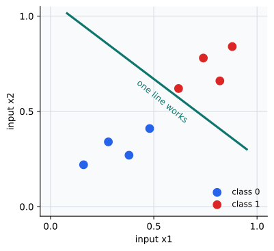
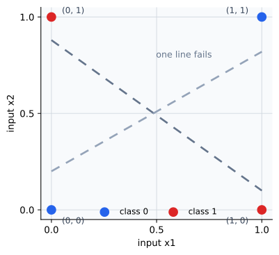
These two graphics are not meant to explain XOR in full yet. They are here to fix what the phrase one linear boundary means in the actual input space. The first figure shows how one line really separates two classes. The second shows separately that even when the rule can be described in a short sentence, one perceptron struggles if the point layout does not split cleanly with one line.
Why Is Activation Needed
If only the linear combination is examined, the result is still just a number \(z\). But what we usually want is one of the following.
- Is it 0 or 1?
- Is it approve or reject?
- Does it react or not react?
The step that turns the score into an actual decision is activation.
In early perceptron explanations, it is often described through a threshold rule.
- If the score is greater than the standard, output 1
- otherwise, output 0
So activation is the step that turns the calculated score into an output rule.
flowchart TD
  A["weighted sum z"]
  B["activation rule<br/>compare with threshold"]
  C["output<br/>0 or 1"]

  A --> B
  B --> C
The result to confirm in this diagram is that the step that creates the score z and the step that turns that score into an actual output such as 0 or 1 are different from each other. So the perceptron should be understood not as a simple adder, but as a sum + decision unit.
Because of this structure, the perceptron is not just a simple adder. It becomes a sum + decision unit.
Cases and Examples
Case 1. Maintenance-Work Resume Score
Let us simplify the judgment about resuming maintenance work. A person first forms an overall impression by looking together at conditions such as isolation valve check, residual gas alarm, and work permit approval. But those conditions have different directions and strengths. Isolation-valve confirmation and permit approval push toward resume, while the residual gas alarm can work strongly in the opposite direction. The linear combination gathers these different signals onto one score axis and starts letting us read whether the work is closer to resume or closer to hold. So the result to confirm in this case is whether comparing resume and hold becomes clearer when several signals are gathered onto one score axis rather than viewed separately.
| Work scene | Isolation valve check contribution | Residual gas alarm contribution | Work permit contribution | Interpretation of the summed score |
|---|---|---|---|---|
| A | +0.9 | 0.0 | +0.5 | It leans toward resume |
| B | +0.9 | -1.2 | +0.5 | It is pushed toward hold |
What matters in this short example is that each condition is not written as a separate conclusion. Instead, all signals begin to be read through one summed score.
Scene A leans toward resume because the safety-check and permit-approval signals work more strongly than the hold signal. In scene B, even if some items look acceptable, the negative contribution of the residual gas alarm presses down the other approval signals and moves the result toward hold. What the linear combination does here is not to list the impressions of the two scenes, but to separate which input actually pushed the boundary.
Case 2. Threshold Judgment for Automatic Blocking
The same score may still not be used directly as an operation command. For example, suppose an automatic blocking system keeps the block in place if z > 0.5, and otherwise passes the case to on-site rechecking. A person might read both 1.4 and 0.6 as toward keeping the block, and both 0.2 and -0.3 as toward rechecking. Here, activation is the step that turns a continuous score into an actual decision rule. In other words, if the linear combination gathers how strongly the situation leans toward keeping the block into a score, activation closes the question so should the automatic block actually remain or not? based on that score. So the result to confirm in this case is whether scores with a similar direction are grouped into the same operational decision.
Score z | Interpretation before activation | After applying the threshold |
|---|---|---|
| 1.4 | Strong keep-block signal | Keep block |
| 0.6 | Weak keep-block signal | Keep block |
| 0.2 | Recheck signal below the boundary | Recheck |
The result to confirm here is that the size of the score and the final decision rule are not the same thing. The linear combination creates direction and strength, while activation folds that score into an actual output category.
From the viewpoint of activation, even if 1.4 and 0.6 both close as keep block, they are not the same signal. 1.4 is a strong block signal, while 0.6 is a weak signal that only slightly crossed the threshold. By contrast, 0.2 may feel positive, but if it does not exceed the threshold of 0.5, the final output still folds into the recheck side. The score is a continuous value, and the decision is the result of folding that score according to a rule.
If the two cases are placed side by side, what a single perceptron actually changes is the way we reread a list of conditions as a score axis and a boundary judgment.
In the maintenance-work resume case, the sum of positive and negative contributions creates a position between resume and hold. In the automatic-blocking case, whether the score z exceeds the threshold 0.5 closes the final output. In both cases, the first result the reader should hold is that the core of the perceptron is not looking at many conditions, but gathering conditions onto one score axis and checking whether that score crosses the boundary.
Why Repeating Only Linear Combination Is Not Enough
At this point, one important deep-learning intuition appears.
Even if a linear combination is repeated many times, the whole result can still collapse back into a linear combination.
There is no need to prove this very strictly here. But the feeling of distinguishing a problem that can be divided by one line from a problem that needs several bent boundaries must be fixed first.
- A problem that can be divided by one line is represented relatively well by one perceptron.
- But a problem with a curved boundary, a boundary split into several pieces, or intertwined conditions is difficult for one perceptron.
In other words, one reason deep learning becomes deep is that more complex boundaries and representations are needed.
Why Does XOR Appear So Often
The XOR problem appears often when explaining the limit of the perceptron. The reason is simple.
XOR is the rule that becomes 1 only when the two inputs are different.
| x1 | x2 | XOR output |
|---|---|---|
| 0 | 0 | 0 |
| 0 | 1 | 1 |
| 1 | 0 | 1 |
| 1 | 1 | 0 |
When people see this table, they often think first, the rule is simple, so maybe one line can separate it too. But once the actual layout is placed as points, the two points that should become 1 lie diagonally apart, so it is hard to divide them neatly with one straight line. In other words, it is a representative case that is not well expressed by the single linear boundary created by one perceptron. The standard people used was is the rule description short?, but from the model's viewpoint the more important standard is can it be divided by one straight line? Because of that difference, a rule can look simple while the expression is still difficult.
It is enough to understand it roughly like this.
Because one perceptron can create only one straight-line boundary at a time, it reveals its limit on patterns such as XOR, which are simple but difficult to separate linearly.
If this is reduced very simply into a diagram, it becomes the following.
flowchart TB
  A["single perceptron"]
  B["one linear boundary"]
  C["works for linearly separable patterns"]
  D["struggles with XOR-like patterns"]

  A --> B --> C
  B --> D
The result to confirm in this diagram is that a single perceptron can make only one linear boundary at a time, so it immediately reveals its limit on problems such as XOR, where the rule description is short but one line still does not separate the points cleanly.
Then What Does a Multilayer Structure Add
This is exactly where the multilayer neural network of Chapter 2 becomes necessary.
If one perceptron creates one straight line, a neural network with several stacked layers can build more complex expressions by combining simple linear decisions several times.
So it is understood through the following flow.
- First, look at one perceptron.
- Next, look at linear combination and activation.
- Then, look at a simple boundary.
- Finally, move toward stacking several layers to create a more complex expression.
This connection is the starting point of deep learning.
Practice and Exercise
The goal of this exercise is not only to see with your own eyes that the linear combination first creates a score, and activation then turns that score into a decision. It is also to explore directly where the boundary actually flips when one value is moved. Compared with calculating the same expression once, it connects more directly to the core of this section to watch the scene where the boundary moves while changing inputs, bias, and threshold little by little.
There are three values to manipulate in this experiment.
alarm_risk: how quickly the score drops as the alarm-risk signal becomes largerb: how strictly or loosely the baseline movesthreshold: where the final decision rule cuts off even for the same score
There are two outputs to observe.
- the linear-combination score
z - the final output after comparison with the threshold
Before the experiment, first predict the change through the following table.
| Value manipulated | Change to expect first | Reason |
|---|---|---|
Increase alarm_risk | z may drop and fall below the boundary more quickly | The input has a negative weight, so the penalty grows as the risk signal grows |
Make b smaller | The same input leads to a more conservative decision | The bias pulls the whole score downward |
Raise threshold | Holds increase while passes decrease for the same z | The activation rule itself becomes stricter |
Now actually change the values. The code below fixes stability_score and shows line by line where the output flips while combining alarm_risk, b, and threshold.
For example, it can be read like this.
This example is a scene where the values change step by step according to the formula. First there is the original input. Next that input becomes the linear-combination score z. Finally it is folded into an output after comparison with the threshold.
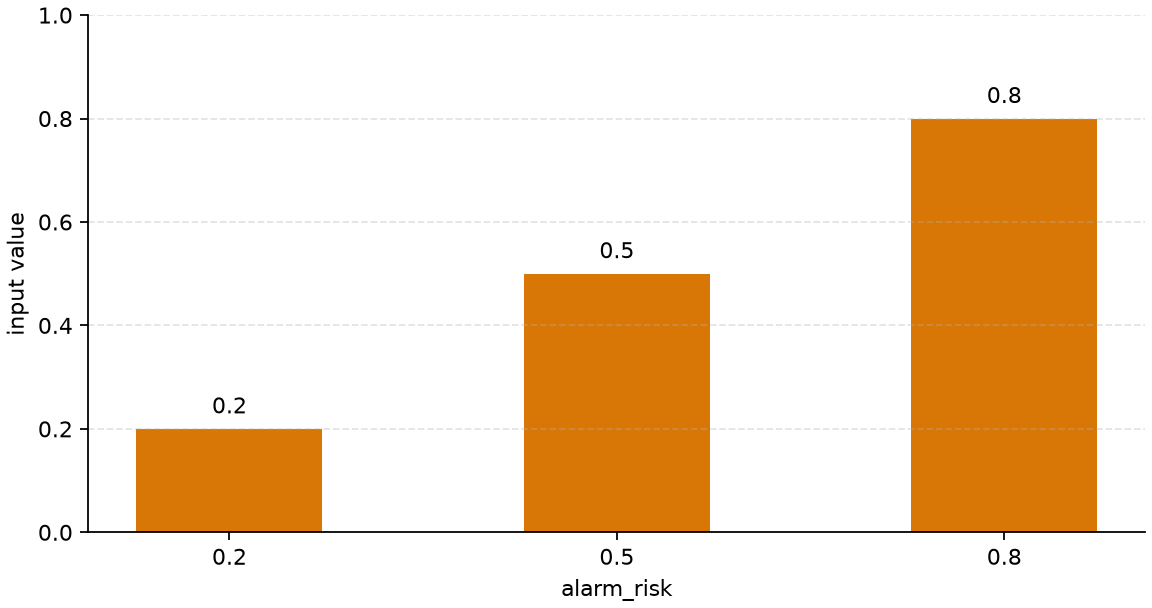
The first graph is the original input changed in the experiment. alarm_risk is still only the size of the danger signal itself, and this value alone does not yet decide whether the final output is pass or hold.
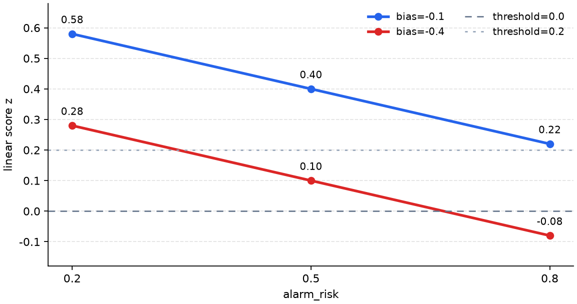
The second graph shows the value after the same input is turned into the linear-combination score z. As alarm_risk grows, the negative weight pushes z downward, and under bias=-0.4 the same input moves to a lower score. Up to this point it is still not the final output, but a continuous intermediate score to compare with the boundary.
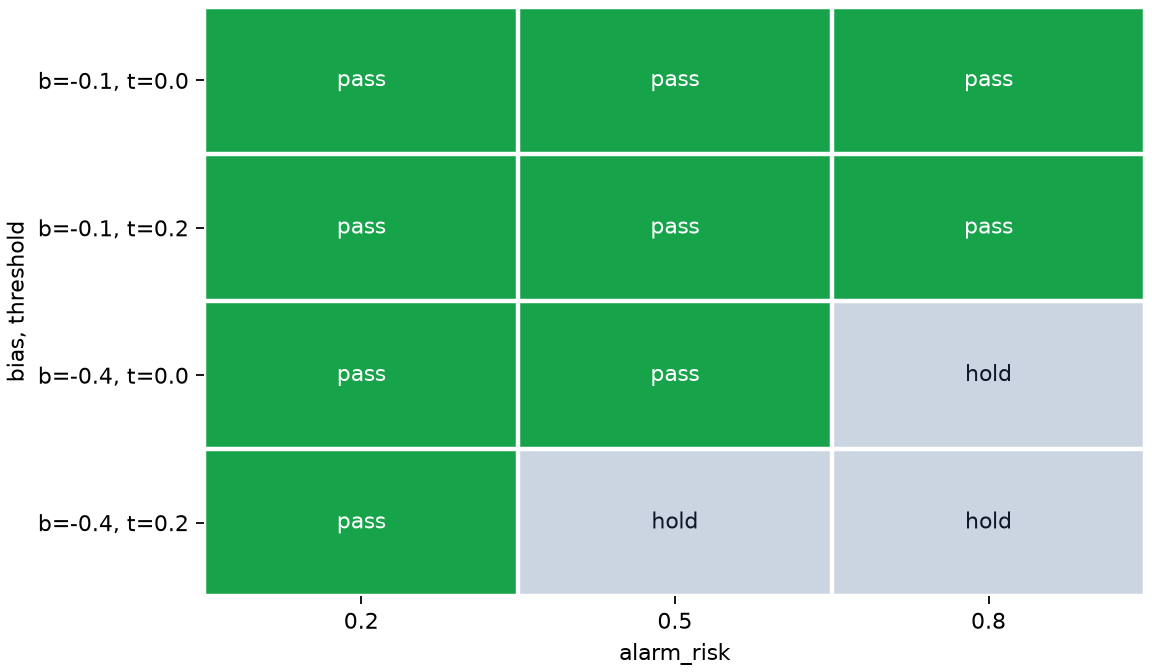
The third graph is the final output after comparing z with the threshold. Even with the same flow of z, passes decrease when the threshold is raised, and a lower bias changes the result to hold earlier in the input range. So the change to confirm in this example is not the input value itself, but the change in meaning along input value -> linear-combination score -> threshold-comparison result.
What should be read first in this output is not an answer table, but which value moved the boundary.
- As
alarm_riskincreases,zfalls little by little. - Even with the same
alarm_risk, loweringbto-0.4makes the result fall below the boundary more quickly. - Even with the same
z, raisingthresholdto0.2changes the output to0earlier.
In other words, the linear combination creates how far and in which direction the score moved, and activation decides so where should it be cut.
If the observation results are organized once more into a table, they become the following.
| What changed in the experiment | Stage that changed directly | Result to confirm in the output |
|---|---|---|
alarm_risk increases | linear-combination score z | As the danger signal grows, the score falls |
b decreases | linear-combination score z | Even with the same input, the boundary moves more conservatively |
threshold increases | activation rule | Even with the same score, pass becomes later and hold becomes earlier |
It is better to change the values one line at a time after running the code once. That makes it clearer what the linear combination moved and what activation moved.
| Value to change next by hand | Output to inspect first | Interpretation question |
|---|---|---|
Add 1.0 to alarm_risks | Under which combination of bias and threshold does output = 0 happen first? | As the danger signal grows, which setting moves the boundary more sensitively? |
Lower stability_score to 0.7 | How much more quickly does z fall even for the same alarm_risk? | Which acted more strongly: the increase in danger signal or the weakening of the stability signal? |
Add -0.1 to thresholds | How much more often does pass appear even for the same z? | Does it become visible that the decision rule can change without changing the score itself? |
By the end of this experiment, the core of linear combination and activation is not I calculated the formula once, but I can explain where the boundary flips when I change the input, bias, or decision rule.
If you recall the linear regression and logistic regression seen in Part 4, the perceptron is not a completely unfamiliar structure. The skeleton is already from the same family: multiply inputs and weights, add them together, add a bias, and connect the result to an output rule. What newly attaches in Part 5 is that this structure repeats as layers, and that activation adds nonlinearity so that more complex representations become possible. In other words, it is enough to remember the perceptron as the first stepping stone that carries the feel of Part 4's linear models into Part 5's neural-network perspective.
Checklist
- Can you explain the linear combination as
a calculation that gathers several input signals onto one score axis? - Can you say that the weight controls the direction and size of each input's influence, and that the bias adjusts the position of the boundary?
- Can you distinguish that activation does not use the score
zitself as the output, but is the step that passes that score through a decision rule? - Can you explain that one perceptron is a classifier that divides the input space at once with one linear boundary?
- Can you say that there are patterns such as XOR whose rule description is short but are still hard to separate with one linear boundary?
- Can you explain why the limit of one perceptron leads to the need for a multilayer structure?
- When the flow of first gathering inputs into one score and then making a decision becomes confusing, can you first recall the two steps of linear combination and activation?
- Do you understand the flow that when one linear boundary is not enough, the next step is to move to the multilayer neural network of the next chapter?
Sources and References
- Frank Rosenblatt,
The Perceptron: A Probabilistic Model for Information Storage and Organization in the Brain, Psychological Review, 1958, date checked: 2026-07-19. https://doi.org/10.1037/h0042519 - Marvin Minsky, Seymour Papert,
Perceptrons: An Introduction to Computational Geometry, MIT Press, 1969/1988, date checked: 2026-07-19. https://mitpress.mit.edu/9780262534772/perceptrons/ - Ian Goodfellow, Yoshua Bengio, Aaron Courville,
Deep Learning, MIT Press, 2016, date checked: 2026-06-28. https://www.deeplearningbook.org/