P5-2.1 Multilayer Neural Networks
Section ID:
P5-2.1Version:v2026.07.26
In P5-1.2, we saw that a single perceptron makes a decision through a linear combination of inputs and activation. At the same time, we also saw that one perceptron can create only one linear boundary at a time, so there is a limit to the patterns it can express. The next question naturally becomes if one perceptron is not enough, what changes if several such computation units are stacked? That question leads into the multilayer neural network. A multilayer neural network is a structure that stacks several computation units like perceptrons across multiple layers, turns simple input combinations into intermediate representations, and then connects those representations to more complex decisions.
When the distinction between multilayer structure and intermediate layers needs to be fixed again, it helps to reread the multilayer neural network and hidden layer entries together in the concept glossary.
Questions Raised by Adding Layers
This section organizes the following questions.
- Why is one perceptron not enough?
- What does it mean to stack more layers?
- How should the input layer, hidden layer, and output layer be read differently?
- What does it mean to say that a multilayer structure creates more complex representations?
- Why is the multilayer neural network treated like the starting point of deep learning?
How a hidden layer can be read as creating real representations continues further in P5-2.2. Comparisons among activation functions reconnect from P5-3.1 through P5-3.5. The computation formulas of backpropagation return in P5-5.1 and P5-5.2. In other words, this section is the place to first hold onto what changes when more layers are stacked and why the hidden layer is needed.
Standards for Multilayer Structure and Expressive Power
- You can explain a multilayer neural network as
a structure that stacks perceptrons across several layers. - You can say that the hidden layer is responsible for intermediate representations between input and output.
- You can understand that a multilayer structure can express more complex boundaries and patterns than a single perceptron.
- You can explain where the split begins between the linear models of Part 4 and the deeper models of Part 5.
Why Add More Layers
One perceptron was already a useful computation unit.
- It receives inputs.
- It creates a weighted sum.
- It produces an output through activation.
The problem is that this one unit alone has difficulty expressing complex patterns.
For example, the following often happens in real problems.
- Input features are not separated by just one simple line.
- Important conditions must be combined across several stages.
- Low-level signals must first be grouped, and then those groups must be combined again into larger meaning.
In other words, if one perceptron is left to make the final decision immediately, too much work is being assigned to it at once.
A multilayer neural network divides this problem structurally.
- The first layer creates small combinations.
- The middle layers regroup those combinations.
- The last layer connects them to the final decision.
The difference becomes clearer if this is moved into a scene of judging abnormality in a small production batch. If x1 alone is high and x2 alone is high are both read immediately through one perceptron, they both tend to collapse first into the question which way should one score lean? By contrast, when layers are separated, the first layer can leave behind did signal A turn on first? and did signal B turn on first? separately, and the later layer can regroup them into did the two signals appear together? and connect that to the final decision. In other words, the core of the multilayer structure is not to crush two inputs directly into one score, but to make it possible to separate the combinations that must be seen separately from the combinations that must be seen together.
Seeing a Multilayer Neural Network in One Scene
flowchart TD
  A["input layer<br/>raw values"]
  B["hidden layer 1<br/>small combinations"]
  C["hidden layer 2<br/>richer combinations"]
  D["output layer<br/>final prediction"]

  A --> B
  B --> C
  C --> D
The key point of this diagram is that as the number of layers grows, the structure is not merely doing more calculation. It is creating intermediate representations.
In other words, a multilayer neural network does not send the original input directly to the final decision. It re-represents the input several times in the middle.
How Are the Input Layer, Hidden Layer, and Output Layer Different
Because the names of the layers can sound abstract, it is easier to divide them by role.
| Layer | Easy role |
|---|---|
| input layer | The entrance that receives the original values |
| hidden layer | The calculation region that turns the input into intermediate features |
| output layer | The last region that produces the final prediction or score |
What matters most here is the hidden layer.
The hidden layer is not a feature directly named by a human. It is an intermediate representation that the model creates and uses inside the calculation process. This is exactly why neural networks move in a different direction from the more traditional models in Part 4.
Why Is It Called Hidden
Because of the word hidden, readers can easily imagine the hidden layer as if it were a secret space. But hidden here does not mean mysterious. It is closer to meaning an intermediate calculation layer that is neither the input nor the final output.
That is:
- The input layer contains values we look at directly.
- The output layer contains results we read directly.
- The hidden layer contains representations used internally by the model in between.
So it is often hard for a person to say immediately, this node means exactly this thing. Instead, we examine whether this layer is creating a more useful intermediate representation.
Why Does It Become Possible to Express More Complex Patterns
One perceptron looked at the input through one linear combination and immediately made a decision. In a multilayer structure, by contrast, the output of one layer becomes the input of the next layer.
That means:
- the combination created by the first layer
- can be received by the second layer as if it were a new input
- and then regrouped into a larger pattern
For an image, for example, the intuition can be described like this.
- very low level: lines, corners, brightness differences
- next level: small shape fragments
- higher level: larger part structures
- final level: a judgment closer to a specific object
Of course, this section is not dealing with CNNs yet. The concrete structure of CNNs returns later in P5-11.1 What Is a CNN. But the feeling that small combinations are stacked into larger combinations is needed from now on.
Reading a Multilayer Structure Through a Table-Style Analogy
Something similar can happen even with tabular data.
Suppose we think about production-line batch data.
- input values: number of micro-stops, duration of temperature drift, pressure fluctuation, number of rework calls
- first hidden layer: intermediate combinations such as thermal burden, operating instability, and quality risk
- next layer: larger pattern combinations
- output layer: final predictions such as whether normal continuation is likely or intervention is needed
For example, suppose output is still being maintained, but the duration of temperature drift is getting longer and the number of rework calls is also rising. A person often tries at first to judge by looking at the four numbers separately. But in practice, these numbers are read together more like a batch whose visible output is being maintained but whose internal instability is growing. If the input values are only compared directly, it is easy to miss this kind of combination signal, and different numeric patterns can still mean the same batch state. The hidden layer should be understood as the place that internally creates such intermediate combinations. What matters, however, is that the hidden layer does not literally know the name thermal burden. We describe it that way for intuition, but the actual understanding is that the model creates some intermediate representation internally through combinations of many weights.
There are roughly three ways people tend to read this first. First, they look at the input values separately and judge things like are the stop counts high? and have the rework calls increased? one by one. Second, they attach one rule immediately, such as if temperature drift lasts long, it is risky. Third, they look first only at the final label, such as is it normal, or does it need intervention?
The multilayer structure changes this reading. Instead of reading the input values one by one, it first looks at the intermediate combinations created by several inputs together. Instead of making a decision immediately from one single rule, the earlier layer creates small combinations and the later layer groups them again into a larger state judgment. So compared with a structure that only looks at the final label, it becomes easier to follow why this intervention judgment came out at the level of intermediate representations.
Cases and Examples
Case 1. Judging Combined Abnormality in a Production Batch
Think about judging combined abnormality in a production batch. At first, a person tends to inspect one rule at a time, such as has the temperature drift duration become longer?, have rework calls increased?, or has pressure fluctuation grown larger? But in practice, the need for intervention often grows only when these three conditions appear together. For example, even if output is still maintained, if the temperature drift duration becomes longer and rework calls also increase, the scene is better read as an intermediate combination like thermal burden + operating instability rather than through a single rule. The multilayer structure explains exactly this flow: one layer creates small signal combinations, and the next layer groups them again into a larger state judgment. So the result to confirm in this case is whether the intermediate combination created when several signals appear together separates the need for intervention more clearly than any one individual rule.
| Batch state | Judgment a person is likely to make first | If reread through an intermediate combination | Safer next judgment |
|---|---|---|---|
| Output maintained, temperature drift lengthens, rework calls increase | Output is still coming out, so it seems fine | Thermal burden and operating instability appear together | Check the combined signal before trusting a single indicator |
| Output is moderate, pressure fluctuation increases, no rework calls | It is only a temporary fluctuation | There is a sign of instability, but the quality-risk signal is still weak | Do not conclude immediately that it is abnormal; look for more signals |
| Output decreases, temperature drift lengthens, rework calls increase | All the numbers look bad | Several danger signals overlap in the same direction | Raise it earlier as an intervention target |
flowchart TD
  A["batch signals<br/>temperature drift, pressure swing, rework call"]
  B["single-rule reading<br/>one metric first"]
  C["combined hidden pattern<br/>thermal load + unstable run"]
  D["next check<br/>review intervention priority first"]

  A --> B
  A --> C
  B --> D
  C --> D
This diagram is a short compression of how the two readings diverge even for the same batch signals: look at one indicator first versus group several signals together. It is not a diagram for adding new theory. It is for rereading the decision order just seen in the case above.
Case 2. Early Intuition for Equipment Image Recognition
Something similar happens in equipment image recognition. A person may look at one photo and immediately think of a final label such as mixing tank, pipe module, or control-box scene, but in practice small clues are seen first, such as a valve outline, a warning-light position, or a metal edge. A single perceptron has difficulty handling all of these clues at once, but in a multilayer structure the earlier layers can create small shape combinations and the later layers can group them into larger equipment clues. For example, the pattern of a valve handle and a pipe curve may be caught first, and then the tank body and connection structure may be grouped afterward into a larger scene cue. So the result to confirm in this case is whether the final label becomes more stable only after passing through combinations of small clues.
| Clues seen first | Small combination grouped in an earlier layer | Larger clue read later |
|---|---|---|
| Valve-handle outline, pipe curve | Small pattern forming part of equipment | A larger equipment clue such as a tank connection |
| Warning-light boundary, control-box corner | Part structure forming a control device | A more stable label candidate such as an equipment scene containing an alarm device |
| Pipe-support line segment, tank-body boundary | Partial clue of a pipe module | A judgment closer to the full shape of the pipe module |
It is tempting to read one photo immediately as a final label, but from the viewpoint of a multilayer structure, the flow is to create small clues first and then regroup those clues into larger structures. Clues such as valves, warning lights, and pipes are not the final label itself. They are the material handled by the earlier layers. The final label becomes more stable depending on how those clue combinations activate together in the later layers.
If these two cases are tied into one line, the core of the multilayer neural network remains the same.
It does not send the input values directly to the final judgment. It passes through intermediate combinations and then groups them into larger patterns.
If the two cases are compressed again at once, the first flow for reading a multilayer structure becomes the following.
flowchart TD
    A[Raw input signals] --> B[Single rule is too weak]
    B --> C[Small combinations are formed first]
    C --> D[Larger state pattern is formed next]
    D --> E[Final decision uses the staged combination]

    F[Raw image cues] --> G[Valve, beacon, pipe cues stay separate]
    G --> H[Front layer builds small visual combinations]
    H --> I[Later layer builds larger equipment meaning]
    I --> J[Final label becomes more stable]
This diagram does not try to explain case 1's production-batch combinations and case 2's equipment-image clues all over again. It is here to hold onto once more the common flow shown by both cases: first create small combinations, then regroup those combinations into a larger judgment.
Comparing One Perceptron and a Multilayer Structure
flowchart LR
  subgraph S["single perceptron"]
    direction TB
    S1["input features"]
    S2["one linear score"]
    S3["one activation"]
    S4["final decision right away"]
    SN["hard to form separate intermediate combinations"]
    S1 --> S2 --> S3 --> S4
    S2 -. everything is compressed into one score .-> SN
  end

  subgraph M["multilayer network"]
    direction TB
    M1["input features"]
    M2["small combinations<br/>hidden layer 1"]
    M3["larger combinations<br/>hidden layer 2"]
    M4["final decision"]
    MN["builds intermediate representations in stages"]
    M1 --> M2 --> M3 --> M4
    M2 -. groups small signals first .-> MN
    M3 -. then recombines them into larger patterns .-> MN
  end
The left side connects the input features directly to the final judgment through one linear score and one activation. So even if there are several signals, they are easy to compress first into a single score. The right side first groups the input features into small combinations, then turns those combinations again into larger combinations, and only then reaches the final judgment. People often feel that both structures are similar because both eventually take input and produce an answer, but the real difference lies in what new combinations can be created in the middle. The important change introduced by deep learning is exactly this: intermediate representations can be learned across several stages.
Why the Multilayer Structure Is the Starting Point of Deep Learning
The reason the multilayer neural network is treated as important is that this is where the model begins to move beyond a simple linear boundary and into representation learning.
Many traditional models in Part 4 learn on top of features chosen by humans. Of course, they can still make combinations and splits, but the feeling that intermediate representations are learned across several layers is relatively weak.
By contrast, the multilayer neural network:
- does not use the input as it is
- changes the internal representation across several stages
- and gradually forms a structure that is favorable for the final judgment
Because of that, the multilayer structure looks like the starting point of deep learning.
If this difference is reduced again from the viewpoint of learning responsibility, it becomes simpler. In the feel of the traditional models from Part 4, people decide more of which features to provide and by what rule to separate them. In the feel of the multilayer structure in P5-2.1, the input and output are placed first, and the job of creating intermediate representations in between is entrusted more to the model. So the first distinction to hold in this section is not does the explanation close with one linear boundary?, but when intermediate representations appear, where does the pattern explanation start to close better?
Practice and Exercise
The goal of this exercise is to check directly how hidden-layer patterns diverge when several inputs pass through the same layer structure, and how that difference connects to the final output. In particular, the values are not changed all at once. One value is changed at a time so that the flow input change -> hidden-layer change -> final-judgment change can be followed.
Input:
- four production batches with two input features each
Output:
- the hidden-layer node values for each batch
- the final output for each batch
Problem situation:
- it is necessary to check directly that the two inputs do not go straight to the final output, but are turned into different abnormality combinations while passing through the hidden layer
- if many values are changed at once, it is easy to miss the point where the judgment flips, so only one value is changed at a time
Concepts to confirm:
- a multilayer perceptron does not send the input directly to the output, but goes through one more stage of hidden-node calculation
- even if the final output is the same or different, the role of the layers becomes clearer only when the earlier hidden pattern is examined together
Input:
First, look at the four batches below and predict which one seems likely to make both hidden-layer nodes turn on together. Then check the actual result through the hidden-layer and output-layer weights.
It is even better to make one judgment before looking at the code.
| Batch | Question to predict first | Expected feel for the final output |
|---|---|---|
(1.0, 0.2) | Will only the first hidden node turn on, or will both turn on together? | If only the thermal-burden side turns on, the final judgment still looks weak |
(0.3, 1.0) | Will the second hidden node turn on first? | It is a different hidden pattern, but the final output may still be 0 |
(1.1, 1.0) | Since both signals are large, will both hidden nodes turn on together? | If both combinations are caught together, it is likely to go to final 1 |
(0.1, 0.2) | Will the process end with almost no hidden representation appearing? | If the hidden representation is weak, the final output will likely remain 0 |
After running the four basic batches first, just follow the three steps below in order.
- Raise only
x1inbatch_2and see whether both hidden nodes turn on together. - Raise only
x2inbatch_1and see whether the same(1, 1)combination appears from a different starting point. - Keep the
batch_2inputs the same, change only the output-layer bias, and see whether the hidden layer stays the same while only the final judgment changes.
In the output, compare line by line which hidden pattern each input passes through before reaching the output.
How the input change alters the hidden-layer pattern appears more directly when placed on the input plane.
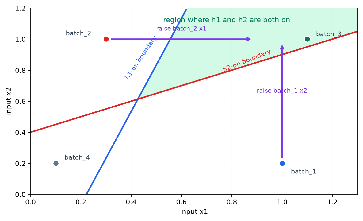
In this graph, the green region is the input area where both h1 and h2 turn on together and lead to final output 1 under the default output-layer bias -0.9. At first, batch_2 stays in the (0, 1) pattern, but when x1 is raised it enters the green region, and batch_1 also moves into the same (1, 1) combination when x2 is raised. By contrast, the step-3 experiment changes only the output-layer bias, so the input coordinates do not move. That case is better read separately through the explanation below than through the graph.
- batch_1 and batch_2 both have final output
0, but their hidden-layer patterns are different:(1, 0)and(0, 1). - Only batch_3 has both hidden nodes turned on and therefore goes to final output
1. - batch_4 barely creates a hidden representation at all, so the final output also remains
0. - In the follow-up experiments, the change can be separated into whether
hiddenchanges first or whether theoutputrule changes first when one input is raised or only the output-layer bias is changed.
It also helps to hold again in a table that even with the same final output, the internal calculation can differ.
| Batch | hidden pattern | output | Core point to read now |
|---|---|---|---|
| batch_1 | (1, 0) | 0 | The first combination alone still does not close the final judgment |
| batch_2 | (0, 1) | 0 | Even if another combination turns on, it may still not be enough |
| batch_3 | (1, 1) | 1 | When both combinations turn on together, the final judgment flips |
| batch_4 | (0, 0) | 0 | If there is almost no intermediate representation, the final result also does not change |
If the same code is run again while changing batch_2's x1 from 0.3 to 0.9, hidden=(0, 1) changes to hidden=(1, 1), and the final output also changes from 0 to 1. In other words, a multilayer neural network has the structure input -> intermediate representation -> final judgment, and the intermediate representation becomes the key material of the real calculation.
Now look directly at the three follow-up experiments below. They let you separate which input change alters the hidden layer from what changes when the decision rule changes even for the same hidden layer.
| Step | Value to change directly | Output to inspect first | Interpretation question |
|---|---|---|---|
| 1 | Raise batch_2's x1 from 0.3 to 0.9 | Does hidden=(0, 1) change into hidden=(1, 1)? | Why does adding more of the first signal flip the final output too? |
| 2 | Raise batch_1's x2 from 0.2 to 1.0 | Does the original (1, 0) pattern extend into (1, 1)? | Even from a different starting point, does adding the second signal complete the same combination? |
| 3 | Keep batch_2's input the same and change only the output-layer bias from -0.9 to -0.5 | Does the output become 1 even with the same hidden=(0, 1)? | Even if the intermediate representation stays the same, can the result change when the final judgment standard becomes looser? |
These three-step experiments separate two kinds of changes.
- Steps 1 and 2 show what new combination the hidden layer starts to create when the input changes.
- Step 3 shows that the result can change even while the intermediate representation stays the same if only the final judgment rule becomes looser.
Even when the starting batches differ, steps 1 and 2 show the shared structure that the final judgment flips when both hidden nodes turn on together. By contrast, in step 3, hidden=(0, 1) stays the same, but the final output changes to 1 because the output-layer standard is relaxed. Once this difference is seen, it becomes clearer that in a multilayer neural network the rule that creates the intermediate representation and the rule that makes the final judgment from that representation must be read separately.
The moment when Part 5 needs to bring in the multilayer neural network is when the calculation of one perceptron is understood, but the explanation of the pattern still does not close with that one linear judgment.
| Problem scene that appears first | Why the multilayer view is useful first | The next question to pass forward immediately |
|---|---|---|
| Several input signals must be combined step by step | It is more natural to distribute intermediate combinations across several layers than to force everything into one score at once. | We need to see what kind of representation those intermediate combinations are actually creating. |
| One linear boundary is too weak to separate the pattern | It shows why the limit of a single perceptron is overcome by expanding the structure. | We must next check why nonlinearity and activation functions are needed. |
| Small clue combinations are needed first in tabular data or images | The flow becomes visible in which the input does not go straight to the final judgment but first creates intermediate material. | We need to see more concretely what the hidden layer is rewriting internally. |
| The split between the linear models of Part 4 and the deep-learning structures of Part 5 must be explained | It reveals most quickly the difference that intermediate representations are learned. | It becomes time to attach the phrase representation learning. |
The core of this section is not the fact that the number of layers increases, but the fact that intermediate representations begin to appear. So the very next section, P5-2.2, continues with what does the hidden layer actually learn?, why is the intermediate representation useful?, and how should we read the change in representation as more layers are crossed? The next question mentioned here is limited not to a theoretical comparison of depth and width, but to the range of reading how several layers change intermediate representations.
| What to hold first in the current section | The question that follows immediately next | The learning-procedure axis that reconnects later |
|---|---|---|
| The fact that the input turns into a larger combination through the hidden layer | What kind of representation can that hidden layer be said to create in practice? | How loss, backpropagation, and the optimizer change that representation |
Checklist
- Can you explain why a multilayer neural network can handle more complex patterns than a single perceptron?
- Can you say through what flow the input layer, hidden layer, and output layer connect?
- Can you explain that a multilayer neural network is a structure that stacks computation units like perceptrons across several layers?
- Can you explain that the hidden layer is responsible for the intermediate representation between input and output?
- Can you say that in a multilayer structure the output of one layer becomes the input of the next, and that this lets the model express more complex patterns and boundaries than a single perceptron?
- Can you distinguish the input layer, hidden layer, and output layer not by
where the data sitsbut bywhat calculation role each layer plays? - When one perceptron no longer closes the explanation and a more complex pattern combination seems necessary, can you think of the multilayer-structure view first?
- Do you know that the explanation of the multilayer structure alone still does not fully close the role of activation functions and nonlinearity, and that these must be passed to the next chapter?
Sources and References
- Ian Goodfellow, Yoshua Bengio, Aaron Courville,
Deep Learning, MIT Press, 2016, date checked: 2026-06-28. https://www.deeplearningbook.org/ - Yann LeCun, Yoshua Bengio, Geoffrey Hinton,
Deep learning, Nature, 2015, date checked: 2026-06-28. https://www.nature.com/articles/nature14539 - George Cybenko,
Approximation by Superpositions of a Sigmoidal Function, Mathematics of Control, Signals, and Systems, 1989, date checked: 2026-07-19. https://doi.org/10.1007/BF02551274