P5-3.1 Activation Functions
Section ID:
P5-3.1Version:v2026.07.26
In P5-2.2, we saw that the hidden layer can turn the input into a more useful internal representation. The next question then appears immediately.
Neural networks are said to do more than simply repeat weighted sums, so what is it that actually creates that change?
The thing that plays that role is the activation function.
An activation function is a function that takes the weighted-sum score \(z\) made by one node and turns it into the value \(a\) that will be passed to the next layer.
In other words, inside one node the following order usually happens: input value -> weighted-sum score z -> activation function f -> value a to pass to the next layer. The activation function is not a separate model that performs learning by itself. It is a transformation rule that changes whether the computed score is passed through as it is, left weakly, or left strongly.
If only this positional relationship is drawn separately, it becomes the following.
flowchart TD
  A["input values"]
  B["weighted sum<br/>score z"]
  C["activation function<br/>f"]
  D["value passed<br/>to next layer a"]

  A --> B
  B --> C
  C --> D
Once this transformation rule makes the relationship depart from a simple proportional line, nonlinearity appears, and the neural network can express more complex patterns.
When the baseline of activation and nonlinearity needs to be fixed briefly again, return to the activation function entry in the concept glossary.
The Question That Needs Activation Functions
- Why is an activation function needed?
- Why is expressive power limited if only linear combinations are repeated?
- What does it mean to add nonlinearity?
- How does the activation function connect to hidden-layer representation?
The differences among representative activation functions continue in P5-3.2 through P5-3.5. The connection between output-layer activation and loss functions returns in P5-3.6, P5-4.1, and P5-4.2. The more detailed context of gradient flow reconnects in P5-5.1 and P5-7.1. In other words, this section first closes why the activation function turns a structure that only repeats linear calculation into real expressive power.
Standards for Nonlinearity and Expressive Power
- You can explain the activation function as
a rule that gives a nonlinear transformation to a score. - You can understand that if only linear combinations are repeated, the whole network can easily collapse back into something linear.
- You can say why the activation function is the key reason multilayer neural networks gain expressive power.
- You can explain, by comparing pre-activation and post-activation values, which signals are cut and which survive.
Why Is An Activation Function Needed
The neural-network computation seen in Chapters 1 and 2 basically has the following structure.
receive inputs -> create a weighted sum -> pass the output to the next layer
The problem is that if every intermediate step is only linear calculation, then even stacking many layers may still fail to make the whole system much more complex.
It is enough to fix it first through the following sentence.
By repeating only linear calculations, it is hard for a neural network to really learn more complex shapes and rules.
So stacking layers alone is not enough. Between the layers, a transformation that bends the straight-line relationship is needed. That transformation is exactly the activation function.
What Does Nonlinearity Mean
Nonlinearity is one of the most abstract words for readers. Here it is enough to understand it first like this.
A property that prevents the output from always changing in direct straight-line proportion just because the input changed a little.
For example:
- if almost no reaction happens below a certain value
- if the response suddenly becomes larger starting from a certain range
- or if signals below a standard are barely passed while signals above it are left more strongly
then the model can now express more complex patterns than a simple straight-line classifier.
Why Is Linear Combination Alone Not Enough
Suppose that linear combinations are repeated across several layers.
- The first layer turns the input into a weighted sum.
- The second layer turns that output into another weighted sum.
But if there is no nonlinear transformation in the middle, these repeated calculations can still be grouped in the end into one larger linear transformation.
That is:
linear combination -> linear combination -> linear combination
If only this is repeated, the depth of the model increased, but its expressive power may not increase as much as expected.
For this reason, the activation function in deep learning is not an optional extra. It is the key device that makes depth meaningful.
If this is drawn very simply, it becomes the following.
flowchart TD
  A["linear layer 1"]
  B["linear layer 2"]
  C["still behaves like a larger linear mapping"]

  A --> B
  B --> C
The result to confirm in this diagram is that even if linear layers are stacked many times, if there is no nonlinear transformation in the middle, the whole thing eventually folds into something like one larger linear calculation, so expressive power does not automatically increase much.
By contrast, once an activation function enters between them, the flow changes.
flowchart TD
  A["linear layer"]
  B["activation<br/>nonlinear transform"]
  C["linear layer"]
  D["richer representation"]

  A --> B
  B --> C
  C --> D
The result to confirm in this diagram is that the activation function inserts a nonlinear transformation between linear calculations, so the next layer can create a more complex representation and connect depth to a real increase in expressive power.
What Does the Activation Function Do to the Score
Let us read again the expression seen above.
- \(z\): the score created by linear combination
- \(f\): the activation function
- \(a\): the new value passed to the next layer
What matters in this section is not memorizing the name of any particular function. It is enough to understand that the activation function does not pass the computed score through unchanged, but changes it into a form that the next layer can use more effectively.
The phrase nonlinear transformation means that it departs from the straight-line rule that if z increases by 1, a also always increases by 1 in the same ratio. For example, consider the following educational rule.
This equation is not here so that you memorize the name of a representative activation function. It is only an example showing that even for the same score \(z\), the degree to which it turns into \(a\) can differ across ranges. In the negative range, the signal weakens. In the middle range, it is passed relatively directly. In the high range, the increase is pressed down again. So the whole graph no longer remains one straight line, but bends in the middle.
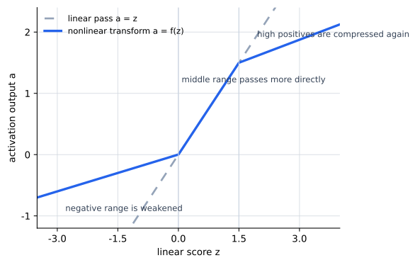
In this graph, the gray dashed line is a linear pass-through such as a = z, where the score is passed unchanged. The blue line is a nonlinear transformation whose response differs by range. To say that the activation function gives a nonlinear transformation means that the value \(a\) received by the next layer is not simply a copy of \(z\), but can become a value whose meaning changes by range in this way.
How Do Hidden Layers and Activation Connect
In P5-2.2, we said that the hidden layer creates an internal representation. The activation function is exactly what keeps that representation from remaining just a simple linear copy.
That is:
- the weighted sum combines the input signals
- activation gives that combination a nonlinear transformation
- and as a result, the next layer can create a more complex internal representation
Because of this connection, the activation function should be read not as a simple output rule, but as a device that makes representation learning possible.
Cases and Examples
Case 1. Classifying Equipment Visual Signals
Suppose an equipment-camera frame must distinguish among a normal piping section, a valve section with the warning light on, and a panel where the pressure-gauge needle has entered the danger zone. People can easily feel that it should be enough just to add together a few edge-like signals that stand out, such as the outline of the warning light, the pipe line, and the frame of the instrument panel.
The first thing to see here is where the activation function enters. Think of one intermediate node receiving visual cues such as the warning-light outline, the needle position, and the circular panel rim, producing a linear score \(z\), and then the activation function turning that \(z\) into the value \(a\) passed to the next layer.
In other words, in this case the activation function is not a device that reads the image directly, but the rule that turns the linear score z made by the intermediate node into the value a that the next layer will read.
For example, this case can be read in the following order.
- In a scene where pipe lines are visible but the combination of warning light and danger needle is weak, the linear score \(z\) tends to remain near a value below the standard.
- If that value is followed after activation, the below-threshold range can almost disappear, so the next layer may not read it as a strong danger signal.
- By contrast, in a scene where the warning-light outline and danger-needle position both appear strongly, the linear score \(z\) rises much higher.
- That scene survives as a larger value even after activation, so the next layer can read it more easily as a
danger combination.
If every calculation stayed linear, then even after stacking several layers, the model could remain something like one large linear filter: if this feature appears a little, add a little to the score. But once activation enters in the middle, some scores are almost cut off while others survive, making it possible to express more complex conditions such as react strongly only when the warning light and needle position appear together. That also helps distinguish scenes where some visual cues overlap, such as pipe curves and circular panel rims.
So the result to confirm in this case is whether scenes that share similar line signals are still separated better into different operational states because the activation function does not copy the linear score \(z\) unchanged, but filters it so that intermediate representations react strongly only to particular combinations.
People often think here only that if a few line signals are visible, the score gets a little larger. But if the scene is reread from the viewpoint of activation, the core is not the amount of cues itself, but which combinations cross the standard and which combinations are almost cut off in the middle. So even when similar line signals such as a pipe curve and a panel rim exist, it becomes possible to form a representation that survives more strongly only for particular combinations.
The core of this case is that visual-cue combinations split into different \(z\) values and different activation results according to weak -> boundary -> strong. In the shared diagram below, this flow is grouped again together with the operational tabular-data case.
Case 2. Operational Tabular Data
Suppose we look together at recent alarm count, pressure-recovery delay time, and restart failure count in an equipment-status table. People can easily feel that simply adding these numbers little by little is enough to read the current danger state.
But even in this scene, the activation function should not be read merely as a justification of necessity. It should be read as the rule that turns the linear score z into the value a that will be passed to the next layer. One intermediate node first receives the alarm count, recovery delay, and failure count, creates the linear score \(z\), and then the activation function turns that value into \(a\).
So in operational tabular data, the activation function is not the rule that reads the table directly, but the rule that decides whether the combined danger score will be ignored by the next layer, remain weakly, or survive strongly.
For example, this case can also be read in the same order.
- A state such as
1 alarm, short recovery delay, 0 failurestends to remain near a below-threshold value if only the linear score \(z\) is examined. - If this value is followed after activation, the below-threshold range can almost disappear, so it may not continue into a strong danger representation in the next layer.
- A state such as
2 alarms, moderate recovery delay, 1 failuremay look, from the linear score alone, like only a slightly larger continuous score. - But if it is followed after activation, this state can be read as a weak signal that barely survives just above the boundary.
- A state such as
4 alarms, long recovery delay, 2 failures, where many signals overlap, not only raises the linear score strongly but also remains as a large value after activation, becoming a danger-combination signal that the next layer should keep paying attention to.
In reality, a bent rule may be needed, such as react strongly as danger only when the alarm count is high and pressure recovery is also slow. If only linear combinations are repeated, every value tends to remain in a simple relationship where it is added little by little. But once activation enters, it becomes possible to form representations that react more strongly only after crossing a particular range, or barely react at all in lower ranges.
Even for the same equipment, if the states are reread across three ranges, it quickly becomes visible why where the representation actually survives matters more than the total sum created by adding little by little. A state with only weak abnormal signals may almost fade if it stays below the standard and may not continue strongly to the next layer. A state that looks ambiguous but slightly more dangerous can remain only barely as a weak signal just above the boundary. By contrast, a state that anyone would judge as clearly dangerous survives as a strong signal that the next layer should keep using.
The difference becomes even clearer if the same input is separated into when only the linear score is examined and when the post-activation value is also examined. If only the linear score is examined, the alarm count, recovery delay, and failure count look like a sum where each signal is added little by little. So it is easy to feel that every signal continues to be reflected only as a continuous score. But once the post-activation value is also examined, the below-threshold range actually weakens almost to nothing, and only certain combinations remain. Only then does the rule the danger representation turns on only when this combination of conditions appears become more directly visible.
In this case too, operational-signal combinations split into different \(z\) values and different activation results according to weak -> boundary -> strong. The case-by-case flow is read through the sentences in the main text, while the diagram compresses only the common signal-survival flow that remains across both cases.
In other words, the activation function can be understood across many data domains as the common device that makes it possible to express more complex rules. So the result to confirm in this case is not a simple summed score where values are added little by little, but whether the danger signal actually reacts more strongly only for specific combinations of conditions.
If the two cases are compressed again into one scene, the flow the reader should hold becomes the following.
flowchart TD
    A[Weak combined signal] --> B[Linear score z stays low]
    B --> C[Activation nearly cuts it]
    C --> D[Little signal reaches next layer]

    E[Borderline combined signal] --> F[Linear score z barely rises]
    F --> G[Activation leaves a small positive]
    G --> H[Weak signal barely survives]

    I[Strong combined signal] --> J[Linear score z rises clearly]
    J --> K[Activation keeps it active]
    K --> L[Strong signal reaches next layer]
This diagram is not intended to redraw separately the visual signals of case 1 and the operational tabular data of case 2. It is intended to let the reader revisit at once the common activation flow shown by both cases: weak -> almost cut, boundary -> remains weakly, strong -> survives strongly.
If this flow is moved into the numerical values used in the exercise, the difference between the pre-activation score \(z\) and the post-activation value \(a\) appears as follows.
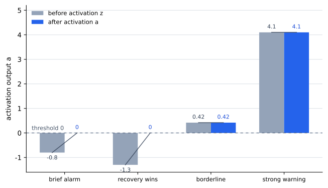
In this graph, the two states that were negative become close to 0 after activation, the signal just above the boundary remains small, and the strong warning signal remains large. Even for the same operational signals, the value actually received by the next layer changes before and after activation.
If the two cases are placed side by side, the role of the activation function does not end at merely making below-threshold signals weaker. In equipment visual-signal classification, a scene that looked like one large score formed by adding line signals little by little can turn, after activation, into an intermediate representation that reacts more strongly only when a particular outline combination such as warning light + gauge needle appears. In operational tabular data, input that looked like a sum where alarm count, recovery delay, and failure count were all added a little at a time can change, after activation, so that below-threshold signals almost fade and only certain condition combinations such as repeated alarm + recovery delay remain more strongly.
The result the reader should hold first here is that the activation function is not merely a device that changes numbers. It is a device that changes what the next layer will look at again as an important signal.
Practice and Exercise
The goal of this exercise is to confirm through case comparison the feeling that an activation function changes a linear-combination score into the value passed to the next layer. Instead of looking at only one input, several operational states are placed side by side so that we can read together which signals survive and which almost disappear.
Input:
- recent alarm count
- pressure-recovery delay score
- restart failure count
- weights corresponding to the three signals
- bias
- four different operational-state cases
Output:
- linear-combination result
z - post-activation result
a - a comparison of which inputs survive and which almost disappear
- a comparison separating weak signals near the boundary from signals that survive strongly
Problem situation:
- it is necessary to check directly how the activation function does not copy the linear score unchanged, but changes which signal will remain for the next layer
Concepts to confirm:
- the activation function does not leave the linear-combination result unchanged, but changes the value passed to the next layer
- if the values before and after activation are placed side by side, it becomes easier to read which signals are actually passed to the next layer
Input:
Following the same flow as the operational-table case, assume that one intermediate node receives recent alarm count, pressure-recovery delay score, and restart failure count and creates the linear score \(z\). Here, the pressure-recovery delay score is not the raw value in actual minutes, but a simplified practice input, roughly between 0 and 3, that becomes larger when recovery is slower.
This exercise uses the following calculation rule.
And the post-activation value \(a\) is read as follows.
This rule is not meant to begin a comparison among representative activation functions. It is a simple rule for experimenting with the feeling that signals below the threshold hardly remain for the next layer, while signals above the threshold remain with differences in size.
First, look at the input values.
| Case | Recent alarm count | Pressure-recovery delay score | Restart failure count | State that a person is likely to read first |
|---|---|---|---|---|
brief_alarm_recovered | 1 | 0.5 | 0 | A state where an alarm appeared briefly but recovered quickly |
recovery_dominant_signal | 0 | 0.5 | 0 | A state where the recovery flow dominates and the danger signal is weak |
borderline_warning_signal | 2 | 2.3 | 0 | A state where alarm and delay overlap and hang near the boundary |
strong_warning_signal | 4 | 3.0 | 2 | A state where repeated alarms, recovery delay, and restart failures overlap together |
It is useful to predict first how each input will look after activation.
| Case | Result to predict first | Reason to expect it |
|---|---|---|
brief_alarm_recovered | z stays below the standard, a hardly remains | Even if there was a brief alarm, if recovery is fast and there are no failures, it is likely to stay below the standard. |
recovery_dominant_signal | z stays below the standard, a hardly remains | If the recovery-delay score is low and there are no failures, it may hardly remain for the next layer. |
borderline_warning_signal | both z and a are weak signals just above the standard | Alarm and delay overlap slightly, so it may sit just above the boundary. |
strong_warning_signal | both z and a are large signals | Repeated alarms, recovery delay, and restart failures overlap together, so they are likely to exceed the standard by a large margin. |
The purpose of this table is not to match the exact decimal values. It is to predict first that the activation function will not copy the linear score unchanged and that a weak signal just above the boundary must be read differently from a sufficiently large signal.
If the same four states are organized through a simple activation viewpoint, they can be read as follows. The values used here are not intended to reproduce exactly the earlier educational piecewise function. They are only a simple observation rule in which below-threshold signals almost disappear and above-threshold signals remain. The goal is not to memorize the name of a particular function, but to see that the pre-activation score z and the value a that actually remains for the next layer do not play the same role.
| Case | z calculation | z | Value after activation | How the next layer reads the state |
|---|---|---|---|---|
brief_alarm_recovered | 0.5*1 + 0.4*0.5 + 1.2*0 - 1.5 | -0.8 | 0.0 | A signal that shook briefly but hardly reaches the next layer |
recovery_dominant_signal | 0.5*0 + 0.4*0.5 + 1.2*0 - 1.5 | -1.3 | 0.0 | A signal that is barely transmitted |
borderline_warning_signal | 0.5*2 + 0.4*2.3 + 1.2*0 - 1.5 | 0.42 | 0.42 | A weak signal that barely survives |
strong_warning_signal | 0.5*4 + 0.4*3.0 + 1.2*2 - 1.5 | 4.1 | 4.1 | A strong signal that the next layer can keep using easily |
If the graph above is read again, the difference in this table becomes visible more quickly. z is the original position created by the linear combination, and a is the position that the next layer actually receives after activation.
If this table is connected again to when only the linear score is examined, the difference becomes even clearer.
When only the linear score is examined, below-threshold values may still look like merely small scores, but after activation brief_alarm_recovered and recovery_dominant_signal actually move close to 0, so they are barely passed to the next layer. By contrast, borderline_warning_signal and strong_warning_signal are both above the standard, but they do not mean the same thing. One is a weak signal that barely survives just above the boundary, while the other is a strong signal that the next layer can keep using easily. This is also why activation makes depth meaningful. It does not stop at comparing the size of linear scores. It actually changes the composition of the next layer's input.
If the interpretation of the output is tied again to real operational judgment, it also becomes visible why the misunderstanding everything above the threshold is the same warning is risky.
If borderline_warning_signal and strong_warning_signal are both read as equally strong warnings, then even weak tracking signals can lead to over-blocking. Both survive, but one is a weak tracking signal while the other is a strong warning signal. By contrast, if brief_alarm_recovered and borderline_warning_signal are both lumped together as ambiguous signals, one misses the difference that one was completely cut off while the other barely survived and still retains tracking value. If a just-above-threshold signal is read as having the same meaning as 0, weak abnormal signs can be missed.
In other words, what should be seen in this section is not the name of any specific representative function, but the fact that activation is the rule that changes where the signal almost disappears, where it survives weakly, and where it remains strongly.
If this is organized once more from the viewpoint of learning, the core of this exercise is not memorizing an answer table. It is being able to explain for yourself where the boundary is, why a just-above-threshold signal must be read differently from a sufficiently large signal, and why the next layer effectively cannot see a signal that almost disappeared.
Finally, change the values directly once more. The table below is a small experiment that can be recalculated by hand.
| Value to change | Case to recalculate | Changed z | Change after activation | Question to raise now |
|---|---|---|---|---|
Lower the bias from -1.5 to -2.0 | borderline_warning_signal | 0.42 -> -0.08 | 0.42 -> 0.0 | If the boundary moves backward, how many weak abnormal signals begin to be missed? |
Raise the restart failure count weight from 1.2 to 1.6 | strong_warning_signal | 4.1 -> 4.9 | 4.1 -> 4.9 | If the intermediate representation becomes more sensitive to failure signals, which cases become stronger? |
Lower the recovery-delay score of borderline_warning_signal from 2.3 to 1.0 | borderline_warning_signal | 0.42 -> -0.1 | 0.42 -> 0.0 | If recovery becomes faster, where should weak warning and normal recovery be separated? |
If only the post-activation value is examined, these three manipulations look as follows.
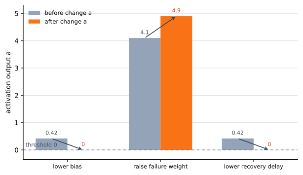
Lowering the bias or reducing the recovery-delay score drops the boundary signal to 0, while increasing the failure weight leaves an already strong signal even larger.
Once this experiment is finished, it becomes possible to confirm that even for the same input, when weights and bias change, the boundary moves, and when the boundary moves, the very signal that remains for the next layer also changes.
Why Does Deep Learning Weaken Without Activation Functions
If there is no activation function:
- the network may look deep
- but the intermediate representation is not bent enough
- and the whole thing can collapse back into one large linear calculation
By contrast, if there is an activation function:
- some signals survive
- some signals are cut
- and the next layer can create more complex combinations
Because of this, the depth of deep learning becomes meaningful only when it is read together with the activation function.
One reason the perceptron and the multilayer neural network regained attention in the history of deep learning also connects to this point. The limit of the single perceptron had been known for a long time, but when multilayer structure, nonlinear activation, and the computational resources and algorithms to train them were brought together again, neural networks began to gain large expressive power.
From the curriculum viewpoint as well, the activation function must appear early. The reason is simple.
- Once you see the perceptron, you understand linear combinations.
- Once you see the multilayer neural network, you understand intermediate representations.
- Once you see the activation function, you understand why that intermediate representation is no longer just a linear copy.
So the activation function is one of the key connecting links in the early part of Part 5.
When Should the Activation-Function View Be Read First
The point where the activation-function section needs to be brought in is when the reason for stacking layers is understood, but why that depth is no longer just a repetition of linear operations is still not closed.
| Problem scene that appears first | Why the activation-function view is useful first | The next question to pass forward immediately |
|---|---|---|
| The explanation is still weak about why repeating linear layers becomes more complex | It shows that nonlinear transformation is the device that turns depth into real expressive power. | We need to see how representative activation functions react differently. |
| It must become clearer why hidden-layer representation is not just a simple copy | It connects the point that after the weighted sum, a rule enters that keeps some values and bends others. | Move on to the differences among representative activation functions. |
| The explanation of multilayer structure risks remaining only an introduction to structure names | The structure begins to be read as computational intuition only after the activation function is attached. | It must later be distinguished from output-layer interpretation. |
| The word nonlinearity still feels too abstract | This is the place where the problem that linear repetition alone is not enough is actually closed. | Concrete function examples should be compared next. |
Checklist
- Can you explain why the activation function is the device that inserts nonlinearity?
- Can you say why depth does not turn into expressive power if there is no activation function?
- Can you explain that the activation function is a rule that gives a nonlinear transformation to a weighted-sum score?
- Can you explain that even if depth increases, expressive power may still not increase enough if only linear combinations are repeated?
- Can you say that the activation function is the key device that lets the hidden layer create a more useful internal representation?
- Can you explain why stacking several layers alone is not enough and why the activation function must be there together?
- Can you describe nonlinearity at least as
the property that prevents everything from following only direct straight-line proportionality? - Before jumping straight into comparing function names, can you use this section as the baseline when you need to regroup why activation is needed?
Sources and References
- Ian Goodfellow, Yoshua Bengio, Aaron Courville,
Deep Learning, MIT Press, 2016, date checked: 2026-06-29. https://www.deeplearningbook.org/ - Yann LeCun, Yoshua Bengio, Geoffrey Hinton,
Deep learning, Nature, 2015, date checked: 2026-06-29. https://www.nature.com/articles/nature14539