P5-3.6 Choosing Output Layers and Activation
Section ID:
P5-3.6Version:v2026.07.26
In P5-3.1, we saw why activation functions are needed, and from P5-3.2 through P5-3.5 we looked separately at the sigmoid, tanh, ReLU, and the formula comparison of representative functions. Once you reach this point, the next question appears naturally.
If functions such as ReLU are often used in the hidden layers, then what activation should be used in the final output layer?
This question connects directly to the loss function. So this section is both the closing part of the activation-function chapter and a bridge into the next chapter.
The activation in the output layer changes depending on what the model is trying to predict, and it is chosen to match what meaning the output value should have.
If the criteria for output interpretation and activation choice become blurry again, reread together the model output, output layer, activation function, and softmax entries in the concept glossary.
The Question of Choosing Output-Layer Activation
- Why should hidden-layer activation and output-layer activation not be treated as the same problem?
- How should the output layer be read in regression, binary classification, and multiclass classification?
- Why must output-layer activation and the loss function be thought about together?
- How should
an output that looks like a probabilitybe distinguished from ascore?
The design of loss functions themselves continues in P5-4.1 and P5-4.2, while the basic reading of calibration and probability-like outputs reconnects in P4-6.4. In other words, this section is the place to first close what unit the final number should be read in for the output-layer activation.
Standards for Prediction Targets and Loss Connections
- You can explain that choosing the output-layer activation connects to
what the model is predicting. - You can read the output layer differently in regression, binary classification, and multiclass classification.
- You can understand that output-layer activation and the loss function do not float separately.
- You can distinguish what unit the final number should be read in depending on the output form.
Why Must Hidden Layers and Output Layers Be Read Differently
Activation in a hidden layer is mainly related to the nonlinearity that makes representation richer. By contrast, activation in the output layer connects more directly to what meaning the final value must carry.
That is:
- hidden-layer activation is closer to a problem of creating internal representation
- output-layer activation is closer to a problem of deciding the interpretation of the final output
Here it is enough to understand it through the following distinction.
The hidden layer changes values in order to create complex patterns, while the output layer matches what those values should mean as a prediction result.
This distinction matters because the roles can easily get mixed under the same name, activation function. In the hidden layer, the central question is can it create a more complex representation? In the output layer, the central question is how should this number be read as a candidate answer? So the choice of output layer is tied more directly to the meaning of the prediction target and the interpretation of the loss than to the convenience of internal computation.
The Output Layer Is Chosen to Match the Prediction Target
If the target that the model is trying to predict changes, then the required form of the final output also changes.
For example:
- if you predict a continuous value such as the total energy use of a mixed batch, then one number can be sent out directly
- if you judge whether a new alarm should trigger immediate shutdown or remain under monitoring, an output that can be read like a value between 0 and 1 may be needed
- if you choose whether a surface-inspection frame is normal, has a fine scratch, or has contamination, then an output is needed that compares several candidates
In other words, the output layer is not just the last node. It is the place where the problem definition decides the shape of the output value.
How Should It Be Read in Regression
In regression problems, the prediction is a continuous numerical value. For example, the model may predict:
- expected energy use of the next batch
- pressure-stabilization completion time
- hourly cooling-water demand
In this case, it is common to leave the output layer as a linear output rather than using a special nonlinear activation. The reason is simple. If the number that must be predicted is unnecessarily compressed into the range between 0 and 1, or between -1 and 1, the expressive range becomes restricted instead.
If a continuous value has to be predicted directly, it is more natural for the output to remain as unchanged as possible.
How Should It Be Read in Binary Classification
Binary classification is the problem of choosing one of two options.
- immediate shutdown / continue monitoring
- remeasurement needed / automatic pass
- overheating risk / normal state
In this case, the sigmoid often appears. Since the sigmoid compresses the output into the range between 0 and 1, it easily gives readers the intuition of a value that can be read like a probability.
But one point has to be handled carefully here.
A sigmoid output is a value that is easy to interpret like a probability. It does not automatically guarantee a perfect probability in every context.
In practice, a threshold policy follows behind it. For example:
- positive if it is 0.5 or higher
- block if it is 0.9 or higher
- review if it is between 0.6 and 0.9
So the number in the output layer and the final service decision must be distinguished.
How Should It Be Read in Multiclass Classification
Multiclass classification is the problem where there are three or more candidates.
- normal / fine scratch / contamination
- pressure recovery / cooling instability / sensor abnormality
- early warning / field inspection / production stop
In this case, each class often first receives its own score, and then a softmax turns those scores into a form that can be compared as relative proportions.
Here it is enough to understand it first with the following feel.
- each class first has its own score
- softmax compares those scores together and reveals
which side is relatively larger
In other words, multiclass classification should not be read as though each output were interpreted only independently. It should be read as a competition structure among candidates.
If this is drawn very simply, it becomes the following.
flowchart TD
  A["hidden representation"]
  B["class scores<br/>normal, scratch, contamination"]
  C["softmax comparison"]
  D["class probability-like outputs"]

  A --> B
  B --> C
  C --> D
This diagram helps the reader read the multiclass output layer as a structure that creates scores and then compares them. Softmax is not just making the numbers look neat. It is the stage that reveals which class is relatively stronger among the candidates.
Are Score, Logit, and a Probability-Like Value the Same
There are three expressions that often confuse readers here.
- score
- logit
- an output that looks like a probability
In this section, the following distinction is enough.
| Expression | Explanation for readers |
|---|---|
| score | A value created inside the model for comparison |
| logit | The last score before being sent into softmax or sigmoid |
| probability-like output | A value that became easier for people to read after passing through sigmoid or softmax |
This distinction matters because it connects directly to the next chapter on loss functions. Some loss functions are designed to receive logits directly, while others assume activated outputs.
Here it is enough to fix first that a logit is still a score before interpretation, while the value after activation is in a form that is easier for a person to read. Without this distinction, even the same number can easily be confused between a value for internal comparison inside the model and a value that may be read like a probability.
Why Must Output-Layer Activation and Loss Functions Be Read Together
If output-layer activation is chosen alone, the explanation stays only half full. That is because the loss function is the device that reads how far the output differs from the correct answer.
For example:
- in regression, a continuous-value output often connects naturally to mean squared error
- in binary classification, the sigmoid and binary cross-entropy are often mentioned together
- in multiclass classification, softmax and cross-entropy are often mentioned together
The output-layer activation matches the meaning of the output, and the loss function reads the gap from the correct answer based on that meaning.
In other words, it is safer to see the output layer and the loss function not as things to memorize separately, but as a paired design.
Cases and Examples
Case 1. Price Prediction
Suppose you are predicting the final energy use of a mixed batch. What people want to know first in this scene is how many kWh will this batch use?, not the probability that it belongs to some usage range. In other words, the output has to remain as a continuous value such as 12.5kWh, so that it can be compared directly with how far it is from the actual energy use.
In this kind of problem, people usually want to know how much directly, not to select a probability category first. So compared with an output compressed into the range between 0 and 1, it is more natural to leave the usage number itself unchanged. For example, what matters is whether it is closer to 12.0kWh or to 15.0kWh, while an indirect value such as probability of being a high-usage batch = 0.8 is not immediately useful. The important standard here is not which category is it?, but how far is it from the correct number? In this case, a regression output is natural. So the result to confirm in this case is whether the output remains a continuous value that lets the real usage difference be compared directly, rather than a value compressed into something probability-like.
| Misreading that a person is likely to make first | Why it is less good | Better reading |
|---|---|---|
Looking at 12.7 and only deciding whether the usage is generally large or small | It misses the core of regression output, which is the distance from the correct answer | Compare first whether the actual answer was 12.4 or 16.0, and by how large the error is |
Reading 12.7 as if it were the probability of some range | It wrongly turns a continuous-value prediction problem into a category problem | Read the number itself as the prediction and judge it together with the allowed error |
Case 2. Alarm-Blocking Filter
Imagine a scene where a line-control system must decide whether to shut down immediately or keep monitoring when a new alarm appears. Here, what the operator looks at first is not an exact number, but should it be blocked or passed? So an output such as 0.91 is not just a decimal value. It is a score that gets read in the direction there is a high chance it belongs to the immediate-shutdown side. In other words, this problem is closer to reading how strongly does it lean between two choices than to predicting one continuous value directly. For example, a value of 0.91 may lead to an immediate stop, while 0.55 may be sent to field review. So an operational policy tends to attach itself immediately behind the output value. The important point here is that the sigmoid output is not itself the final policy.
But actual operation does not stop there. For example, 0.91 may trigger automatic stop, 0.65 may send the case to field confirmation, and 0.30 may only be logged. So the result to confirm in this case is whether even for the same sigmoid output, the interpretation of the score and the actual processing rule are operating as different stages.
If 0.91 is read immediately as shutdown decision, the model output and the operational policy get lumped together. In reading the output layer, 0.91 should first be seen as the model output, and only after that is the shutdown decision made at the policy stage. Even with the same decimal value, different facilities may use different thresholds, so the interpretation of the sigmoid score and the threshold policy must be examined separately.
Even for the same sigmoid output, some misreadings are comparatively less bad, while others are more dangerous.
| Output scene | Less bad misreading | More dangerous misreading | Better reading |
|---|---|---|---|
0.55 | Read it as leaning positive, but still ambiguous | Decide immediately automatic shutdown | Separate the model output from the operational threshold and look first for an intermediate policy such as field confirmation |
0.91 | Read it only as a strong warning and leave the detailed policy for later | Think that 0.91 itself is the policy and ignore that the threshold can differ by facility | Read it as a strong positive score, but also check where the automatic-shutdown standard is actually placed |
Case 3. Quality-State Classification
Suppose you have a model that automatically classifies a surface-inspection frame as normal, fine scratch, or contamination. People often want to see only one name first, as in what state is it?, but the model first creates a set of competing scores such as normal, scratch, and contamination. What matters here is not only the top-ranked name, but also how far ahead it is.
For example, if the output is normal 0.70, scratch 0.20, contamination 0.10, a person can read it as it leans most strongly toward normal. By contrast, if the output is normal 0.38, scratch 0.34, contamination 0.28, then even if one answer is still chosen, the model's confidence does not look high. At first, people may feel that seeing only the top class name is enough, but in reality how far ahead it is of the others is also important. For example, the decision whether to finalize automatic classification or hand the case to human review can depend heavily on that gap. In this case, a multiclass structure that reads several class scores together is natural. So the result to confirm in this case is whether not only the top class name, but also the score gap from the other candidates remains available for separating automatic processing from human review.
| Output scene | Judgment a person is likely to make first | Why it is insufficient | Better reading |
|---|---|---|---|
normal 0.70, scratch 0.20, contamination 0.10 | normal is ranked first, so confirm it immediately | This may not be a major problem here, but it leaves no standard for why automatic confirmation was acceptable | Also examine that the score gap between the top candidate and the others is sufficiently large |
normal 0.38, scratch 0.34, contamination 0.28 | normal is ranked first, so end it as normal again | The gap among candidates is narrow, so the model confidence is low, but the case may still be finalized automatically | Look first at the lack of score gap rather than the top name, and send it to human recheck |
If the three cases are placed side by side, the choice of output layer becomes a problem not of which function should be attached at the end?, but first of what should the final number be read as?
If the numbers from the cases are fixed again through graphs, the difference becomes clearer. In regression, the first thing seen is how far the prediction is from the actual value.
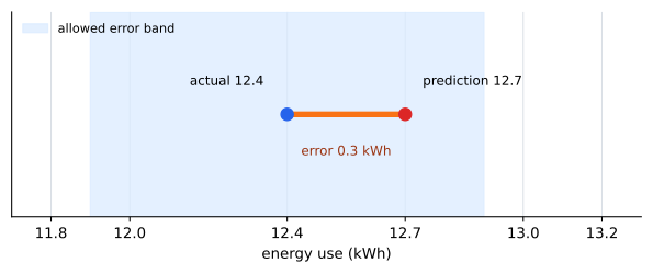
In binary classification, it becomes visible that a score such as 0.91 is not the policy itself, but a model output that lies inside a threshold band.
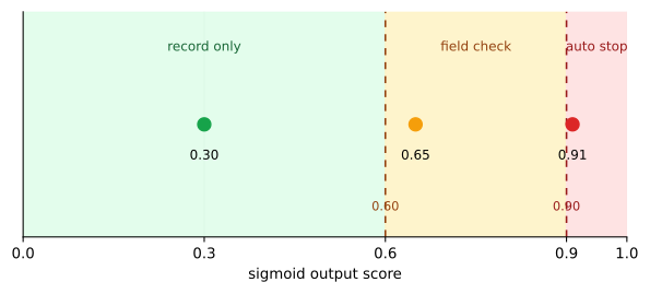
In multiclass classification, instead of looking only at the name of the top candidate, the gap between the first and second candidates must also be examined.
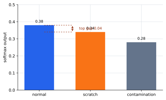
So what should be read first in these graphs is not the decoration of the curves or bars, but the interpretation units: distance for regression, threshold position for binary classification, and gap among candidates for multiclass classification.
| Problem type | Result a person is likely to look at first | Interpretation the output layer actually needs to leave behind | Output feel that connects naturally to the loss |
|---|---|---|---|
| Regression | A continuous number such as how much | A continuous value whose size can be compared directly | Distance from the correct number |
| Binary classification | Two choices such as block or pass | A score between 0 and 1 plus a separate policy behind it | Confidence toward the positive class |
| Multiclass classification | Which name ranks first | Relative comparison among candidates and the score gap | How far ahead the correct class is among several candidates |
What the reader should hold first in this table is that choosing output-layer activation is not choosing a function name, but fixing first the meaning of the final output that will be compared with the correct answer.
Practice and Exercise
Even when the values look like similar numbers, the output layer has to be read differently depending on the problem type. If the following three scenes are placed together, the difference becomes clearer.
| Problem type | Model's final output | Unit to read first | What the loss compares first |
|---|---|---|---|
| Regression | predicted usage = 12.7kWh, correct answer 12.4kWh | Distance from the correct number | Error between the predicted value and the correct value |
| Binary classification | sigmoid output = 0.881, correct answer positive | Threshold band and policy separation | How strongly it leans toward the positive correct class |
| Multiclass classification | normal 0.214, scratch 0.713, contamination 0.072, correct answer scratch | Gap between the top candidate and the others | How far the correct class is ahead of the other candidates |
What must be seen first in this table is that the shape of the output value and the way it is compared to the correct answer are decided together. Regression leaves the number itself alone and looks at the distance from the correct answer. Binary classification reads the output as a score between 0 and 1 and then looks at how strongly that score leans toward the correct class. Multiclass classification must look not only at the top-ranked name, but also at how far the correct class is ahead of the other candidates.
If the same scene is changed a little, it also becomes visible what should be reread first.
| Changed output scene | Standard that should be reread first | Question to raise immediately |
|---|---|---|
A regression output changes from 12.7 to 13.2 | Distance from the correct answer rather than the absolute size of the number | Did it move farther from the correct answer 12.4? |
A binary-classification output falls from 0.881 to 0.61 | Policy threshold and the direction of the score | Does it move down from automatic blocking into the field-confirmation band? |
A multiclass output becomes close, such as 0.38, 0.34, 0.28 | Gap among the candidates rather than the name ranked first | Is manual recheck safer than automatic confirmation? |
In this exercise, the following three questions must be closed directly.
- Why should a regression output such as
12.7be read first through its distance from the correct answer12.4, rather than through something compressed like sigmoid or softmax? - Why should a binary-classification output such as
0.881be read first as a model output lying above a threshold, rather than as the policy itself? - Why, in multiclass classification, is it not enough to stop at the fact that
scratchis ranked first, but necessary also to look at how far ahead it is of the other candidates?
The direction of the answer is clear. In regression, the final number itself is the prediction, so the loss first looks at how far that number is from the correct answer. In binary classification, the sigmoid output shows the direction toward the positive class, so the loss reads that score according to whether the correct answer is positive or negative. In multiclass classification, the candidates compete together, so the loss also connects to whether the correct class is sufficiently ahead of the others.
So the result that the reader should leave with from this exercise is not which activation was used, but in what unit the final number should be read, and what part of that number the loss ends up comparing.
In the educational flow of early neural networks and statistical classification models, how the final output should be read has long been an important topic. The connection between logistic regression and the sigmoid, multiclass probability interpretation, and the coupling with loss functions are all questions that extend from before deep learning.
This is also why this section is needed in the deep-learning curriculum.
- If activation functions are seen only as the nonlinearity of the hidden layer
- it becomes easy to miss why the final output must change depending on the problem
- and when the loss-function chapter begins, only formulas are left standing suddenly
So this section prepares the next chapter by showing that loss functions are not rules that appear out of nowhere, but design choices connected to output interpretation.
When Should Output-Layer Interpretation Be Separated Out First
Once the explanation of hidden-layer activation is finished, what the final number should mean must be separated out and examined on its own. This section handles exactly that turning point.
First, ask what kind of problem it is. If it is a continuous value, then the final number is read directly as the prediction. If it is a problem of choosing one of two options, then a score between 0 and 1 is read together with the threshold policy. If several classes are competing, do not look only at the top name; read the candidate scores and score gaps together. Only after this interpretation is fixed does the standard for how the loss function reads how far it differs from the correct answer become fixed as well.
flowchart TD
  A["What is the prediction target?"]
  B["continuous value"]
  C["one of two choices"]
  D["one of several classes"]
  E["keep the number as a value"]
  F["read a 0-1 score<br/>with a threshold policy"]
  G["compare class scores<br/>and the margin"]
  H["connect to the matching loss"]

  A --> B
  A --> C
  A --> D
  B --> E
  C --> F
  D --> G
  E --> H
  F --> H
  G --> H
The point that especially needs care in this flow is the case where service policy and model score are read together as one thing. The model output is the final value to compare with the correct answer, while operational decisions such as automatic blocking, field confirmation, and human review come afterward. Only if output-layer interpretation is separated first can the loss function and evaluation criteria in Chapter 4 also continue on the same unit.
Checklist
- Can you explain that choosing the output-layer activation connects to the meaning of the prediction target?
- Can you say why hidden-layer activation and output-layer activation are not treated as the same problem?
- Can you explain that hidden-layer activation and output-layer activation have different roles?
- Can you say that output-layer activation should be chosen to match the problem type and the interpretation of the output?
- Can you explain how the output should be interpreted in regression, binary classification, and multiclass classification?
- Can you explain that output-layer activation and the loss function naturally need to be designed together?
- When you find yourself explaining hidden layers and output layers the same way just because they both use activation functions, can you separate out the problem of output interpretation first?
- When it is easy to mistake sigmoid or softmax output for the service policy itself, can you bring out the view that separates model score from operational decision?
Sources and References
- Ian Goodfellow, Yoshua Bengio, Aaron Courville,
Deep Learning, MIT Press, 2016, date checked: 2026-06-29. https://www.deeplearningbook.org/ - Christopher M. Bishop,
Pattern Recognition and Machine Learning, Springer, 2006, date checked: 2026-07-19. https://link.springer.com/book/9780387310732 - Kevin P. Murphy,
Probabilistic Machine Learning: An Introduction, MIT Press, 2022, date checked: 2026-07-19. https://probml.github.io/pml-book/book1.html