P5-4.1 Loss Functions
Section ID:
P5-4.1Version:v2026.07.26
In Chapter 3, we saw that activation functions insert nonlinearity into neural networks and increase expressive power. The next question then follows immediately.
How, then, does a neural network judge how wrong its current output is?
The standard that answers this question is the loss function.
A loss function is the rule that turns how far the model's current output differs from the target into one number.
However, textbooks and framework documents sometimes separate loss from objective or cost a little more carefully. Often, loss refers to the per-sample discrepancy or its average, while the full target that is actually minimized is explained as an objective/cost that includes the batch average together with regularization. In this section, for beginner flow, everything is first explained under the single name loss, but when gradients and the optimizer are connected in later sections, we return to the question what is actually being minimized?
When the role of loss needs to be checked again briefly in later sections, return to the loss function, metric, squared error, and cross-entropy entries in the concept glossary.
Here it is enough to fix the following three sentences first.
- Learning has not started yet if we only look at the output.
- The mistake must be turned into a number before the next calculation can continue.
- That number is exactly the loss.
The Question That Needs Loss Functions
- What does the loss turn into a number?
- Why does the loss function become the central standard in deep learning?
- How is the loss function different from an evaluation metric?
- What does it mean in learning when the loss value becomes smaller?
The concrete kinds of loss functions and their differences by problem type continue in P5-4.2, while how differentiation and gradient calculation actually connect to backpropagation returns in P5-5.1 and P5-5.2. In other words, this section is the place to first hold onto the role of loss as turning the gap between prediction and target into a number that learning can use.
Standards for Reading Error as a Number
- You can explain the loss function as
the standard that turns the current prediction error into a number. - You can distinguish the loss function from an evaluation metric.
- You can explain what it means in learning to reduce the loss.
- You can explain which wrong answers the difference between prediction and target causes the model to correct more strongly first.
Why Is a Loss Function Needed
Neural networks produce outputs. But output alone does not yet make learning happen. The model has to be able to ask itself:
How bad is the current result?
If that question is not turned into a number, the next step is impossible.
- The model does not know in which direction the weights should change.
- It does not know whether the current model is better than the previous one.
- It becomes hard to compare which output candidate is worse than another.
In other words, the loss function is the reference point by which the neural network checks its own result.
This scene can be restated as follows.
Without loss, the model cannot compare for itself whether things have become better or worse.
What Does Loss Measure
Loss usually compares the following two things.
- the current output made by the model
- the target we expected
It is enough to understand it like this.
Loss is a number that compresses the gap between prediction and target.
For example:
- if the correct answer is 10 and the prediction is 9, the loss may be relatively small
- if the correct answer is 10 and the prediction is 2, the loss may be larger
In other words, loss does not stop at simply right or wrong. It lets us read how far it is off through a more continuous number.
An important feeling readers often gain here is the following.
- whether it is classification or regression, loss deals with
the degree of wrongness - loss usually gives a smoother number than a hard judgment such as
0 or 1 - and precisely because of that, gradients can later be calculated
If this flow is compressed very briefly, it becomes the following.
flowchart TD
  A["Model prediction"]
  B["Target"]
  C["Compare the gap"]
  D["Loss value"]
  E["Gradient signal"]
  F["Parameter update"]

  A --> C
  B --> C
  C --> D
  D --> E
  E --> F
The result to confirm first in this diagram is that loss is not just a bad score, but the connection point that passes the difference between prediction and target into the next update.
How Is It Different from the Metric in Part 4
In Part 4, we looked at evaluation metrics such as accuracy, precision, recall, F1, and RMSE. At this point, it is easy to understand the loss function and the evaluation metric as though they were the same thing.
But the two have different roles.
| Category | Loss function | Evaluation metric |
|---|---|---|
| Main role | Internal standard for learning | Standard for evaluation and selection |
| Time of use | Used continuously during learning | Used for mid-training checks, early stopping, and final evaluation |
| Question | How wrong is it right now? | How well did it actually perform? |
So it is better first to distinguish that the loss function is the standard by which the model learns, while the metric is the standard by which the model is evaluated and selected.
Of course, the two are not completely separate. A good loss design should usually connect in some way to the performance direction we care about. But the two do not have the same role.
Why Is Loss Gathered into One Number
Neural networks have many parameters. In order to change those parameters, the current state has to be gathered into one comparable standard.
For example, across several samples:
- some predictions may be slightly wrong
- some predictions may be very wrong
- some predictions may be almost correct
If that state is left as it is, it becomes hard to decide an update direction. So the loss function gathers many discrepancies into something like one number. In actual learning code, that number is reduced into a batch average or sum, and sometimes a regularization term is added so that the whole thing becomes the full objective/cost that is optimized.
In other words, the loss function plays the role of the compass number of the learning process.
If this is reduced into one sentence for readers, it can be remembered like this.
Loss is the signal that compresses into one number the direction in which the model is currently going wrong.
What Does It Mean When the Loss Decreases
This can be explained by the following sentence.
When the loss decreases, it means that the current model is creating less discrepancy from the target, at least on the training data.
But even here there is a point that needs care.
- just because the training loss decreased
- it cannot be concluded immediately that generalization improved
This point connects directly to the explanation of overfitting and generalization in Part 4. In other words, loss is very important, but the whole model cannot be judged from loss alone.
Cases and Examples
Case 1. Predicting Batch Energy Use
Suppose we are predicting the total energy use of one mixed batch. If the actual usage is 5.0kWh, model prediction A is 4.8kWh, and model prediction B is 2.0kWh, then a person first looks at which one is closer to the actual usage? Even by that standard alone, it is immediately visible that prediction A is less wrong than prediction B. But learning has to repeat this judgment with the same rule across all samples, so slightly off and far off must be turned into consistent numbers. The loss function turns exactly that difference into numbers that learning can use, so that it becomes possible to compare which prediction is worse and which is less bad. In other words, in regression problems, the first task is to turn how far off is it? into a number, rather than merely is it wrong?
| Comparison item | Prediction A | Prediction B | Core point to read now |
|---|---|---|---|
| Difference from actual usage | 5.0 - 4.8 = 0.2 | 5.0 - 2.0 = 3.0 | Both are wrong answers, but the degree of error is completely different. |
| Judgment a person is likely to make first | Almost correct | Very wrong | The difference is intuitively visible, but learning needs that difference to remain as a repeatable number. |
| From the viewpoint of loss | Small penalty | Large penalty | The loss function spreads apart a less bad wrong answer and a much worse wrong answer numerically. |
If the same difference is read through the simplest rule, such as squared error, it becomes immediately visible why the loss spreads out.
| Example of loss calculation | Prediction A | Prediction B | Result to confirm now |
|---|---|---|---|
| Error | 4.8 - 5.0 = -0.2 | 2.0 - 5.0 = -3.0 | The direction is the same in both cases, predicted lower than actual, but the size is very different. |
| Squared error | (-0.2)^2 = 0.04 | (-3.0)^2 = 9.0 | The loss of B spreads much more than that of A. |
| Interpretation of the update signal | A state that needs only a small adjustment | A state that needs a large correction | The larger the loss number becomes, the clearer it gets which prediction should be corrected more strongly first. |
| Standard a person is likely to look at first | Standard reread from the viewpoint of loss |
|---|---|
| Just see that neither one is exactly correct | Even among wrong answers, the one that missed by a larger amount has to be spread farther apart numerically |
| Keep only the feeling that A is better than B | That feeling must be turned into a loss number that can be repeated across all samples |
| In regression, it is easy to feel that being approximate is enough | Learning has to read how close was it? as a continuous value before an update direction appears |
The final result to confirm in this case is clear. Even if both predictions are wrong, loss does not stop at both are wrong. It gives a much larger number to prediction B, which missed by more, so that it will be corrected more strongly first.
Case 2. Classifying Inspection States
Classification works similarly. Suppose the correct answer is fine scratch, but model output A is normal 0.51, fine scratch 0.49, and model output B is normal 0.99, fine scratch 0.01.
People can easily say that both are wrong and move on. But from the viewpoint of learning, those two wrong answers cannot have the same weight. A almost got it right, while B judged the opposite very confidently. So the loss function also reflects how confidently it was wrong, and distinguishes cases where the same wrong answer still needs a much stronger correction. In other words, in classification problems, more than simple right-or-wrong, it also matters with what confidence did the model get it wrong? So the result to confirm in this case is whether, even though both are wrong answers, B receives a much larger penalty in the loss because it predicted the opposite with confidence.
| Comparison item | Output A | Output B | Core point to read now |
|---|---|---|---|
| Predicted label | normal | normal | If only the final label is looked at, both are the same wrong answer. |
Probability for the correct answer fine scratch | 0.49 | 0.01 | A almost got it right, but B gave almost no probability to the correct answer. |
| Judgment a person is likely to make first | Wrong | Wrong | If we look only at right or wrong, the difference between the two disappears. |
| From the viewpoint of loss | A wrong answer closer to a small penalty | A wrong answer with a much larger penalty | Even among the same wrong answer, loss spreads apart the difference in probability given to the correct answer. |
Even without deriving cross-entropy in detail, the example the lower the probability assigned to the correct answer, the larger the loss becomes can be checked immediately.
| Example of loss calculation | Output A | Output B | Result to confirm now |
|---|---|---|---|
Probability given to the correct answer fine scratch | 0.49 | 0.01 | The loss looks directly at how much probability was given to the correct class. |
Example of cross-entropy loss -log(p) | -log(0.49) ≈ 0.713 | -log(0.01) ≈ 4.605 | The loss of B is much larger than that of A. |
| Interpretation of the update signal | A state where only the boundary may need slight adjustment | A state that needs a large correction toward the correct direction | The more confidently wrong it is, the stronger the correction signal becomes. |
If these two cases are turned back into graph shapes, regression loss grows as it moves farther away from the target value, while classification loss grows as the probability assigned to the correct class becomes smaller.
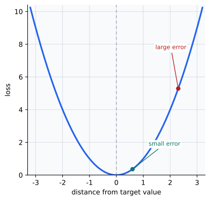
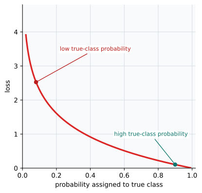
The purpose of these two graphs is not to memorize the formulas. It is to see along which axis does the loss grow larger? In regression, the key axis is the distance from the target value. In classification, it is the probability assigned to the correct class.
| Standard a person is likely to look at first | Standard reread from the viewpoint of loss |
|---|---|
| See both as the same wrong answer | Also look together at how far they are from the correct answer and how confidently they were wrong |
Read 0.51 and 0.99 only as both predicting normal | Separate A as a wrong answer that almost got it right, and B as a wrong answer that was strongly confident in the wrong direction |
| It is easy to feel that a two-step right/wrong judgment is enough | Loss separates the degree of wrong answers more finely into numbers |
The final result to confirm in this case is also clear. In classification, even for the same wrong answer, a prediction such as B, which assigned almost no probability to the correct class, receives a much larger loss and is corrected more strongly first.
The core shown together by these two cases is the same. In regression, how far did it miss? matters more. In classification, how confidently was it wrong? matters more. Those things have to be reflected more strongly in the loss number so that the next update becomes more accurate.
If these two cases are tied into one line, the common role of the loss function is the same.
Turning the model's current discrepancy into a number that learning can use
And in this section, the explanation has to go one step further and close, at the level of cases, why is loss needed separately from the metric?
| Problem type | Result a person is likely to see first | If only the metric or the final right/wrong judgment is seen | What loss additionally reveals | Prediction that should be corrected first |
|---|---|---|---|---|
| Predicting batch energy use | A is closer to the actual usage than B | If all we know is that both are wrong, the update priority is still not clear enough | B missed much farther than A, so the loss spreads much larger | Prediction B |
| Classifying inspection state | Both A and B predicted normal, so both are wrong | From accuracy alone, both may look equally like 0 | B gave almost no probability to the correct answer fine scratch, so the loss is much larger | Output B |
The core this table shows is simple. Even in cases that look like the same wrong answer when we look only at the metric or the final judgment, loss more finely distinguishes which wrong answer is more dangerous and should be corrected more strongly first.
flowchart TD
  A["Results that look equally wrong"]
  B["Human or metric view"]
  C["Both are just wrong or low-scoring"]
  D["Loss view"]
  E["Separate distance and confidence gaps"]
  F["Larger loss gets higher update priority"]

  A --> B
  B --> C
  A --> D
  D --> E
  E --> F
The final result the reader should hold in this flow is that loss is not an auxiliary score added after right/wrong judgment. It is the number that decides update priority.
One reason loss functions always appear early in machine-learning and deep-learning education is that learning is not simply repeating rules, but an optimization problem.
The core flow of deep learning usually continues like this.
put in an input -> create an output -> calculate the loss -> change the parameters in the direction that reduces the loss
In other words, the loss function is not an optional extra attached after the output. It is the standard that starts the whole learning calculation.
From the curriculum viewpoint as well, only when the loss function is understood first does it become natural to read:
- why backpropagation is needed
- what the optimizer is trying to reduce
- what number the learning rate is following
Practice and Exercise
The goal of this exercise is to read the simplest possible process in which the difference between prediction and target turns into a loss number. Rather than looking only at the average loss, the sample-by-sample errors are also checked so that it becomes visible on which item the large error occurred.
Input:
- 3 target values
- 3 prediction values
Output:
- squared error of each sample
- the sample that was most wrong
- average loss
Problem situation:
- the loss function should not be read only through the final average value; it must also be checked how the sample-by-sample errors accumulate
Concepts to confirm:
- average loss is a number made by gathering the error of each sample
- if the sample with the largest error is found, it becomes easier to interpret why the loss became large
Input:
Use the sample-by-sample target values and prediction values organized above.
Before looking at the table, it is useful first to predict which sample will pull up the average loss the most.
| Sample | Loss size to predict first | Reason to expect it |
|---|---|---|
night_shift_batch | Medium | The gap between target 3.0 and prediction 2.5 is 0.5, so it is not completely small. |
stabilized_batch | Smallest | The gap between target 1.0 and prediction 1.4 is 0.4, the smallest of the three samples. |
restart_delay_batch | Largest | The gap between target 2.0 and prediction 1.2 is 0.8, the largest of the three. |
The purpose of this table is not to calculate the exact squared error in advance, but to hold first that average loss is not pulled equally by all samples; it is pulled more by the items that are more wrong.
If the same three batches are organized through the viewpoint of loss, they can be read as follows.
| Sample | target | prediction | squared error | Result to read now |
|---|---|---|---|---|
night_shift_batch | 3.0 | 2.5 | 0.25 | It needs a mild correction, but it is not the highest-priority worst case. |
stabilized_batch | 1.0 | 1.4 | 0.16 | It is the least wrong of the three batches, so its contribution to the loss is the smallest. |
restart_delay_batch | 2.0 | 1.2 | 0.64 | It is the key wrong answer that pulls up the average loss the most. |
If these three values are gathered into the average, mean_loss = 0.35, and the batch that missed the most is read as restart_delay_batch.
What matters in this exercise is how the average loss number 0.35 was made.
- The first sample was slightly wrong.
- The second sample was also slightly wrong.
- The third sample was more wrong.
The loss function gathers these discrepancies into one number so that the model can read how bad its current state is. At the same time, if the sample-by-sample errors are examined, it also becomes visible which case is pulling up the average loss the most.
What the reader must read in this example is the following.
- The degree of error differs by sample.
- The loss function does not discard that difference, but reflects it numerically.
- The mistakes of several samples can be gathered into one average standard.
But if it stops there, it still remains only at the level of I looked at one average loss number. A loss example must also immediately make visible which sample should be corrected more strongly first.
| Output signal | Less bad reading | More dangerous reading | Better next judgment now |
|---|---|---|---|
mean_loss = 0.35 | Read it as the average discrepancy of the three samples at the moment | Decide that the judgment is finished just by looking at 0.35, without deciding which sample to correct | Read that the average is only a summary of the full state, and that the sample-by-sample error breakdown must also be examined before update priority becomes visible |
worst_sample = restart_delay_batch | Read it as the sample that pulls up the average loss the most among the three | Treat restart_delay_batch as if it were only an outlier that can simply be discarded | Reread it as the prediction type that must be corrected first by checking again why restart_delay_batch missed so largely in terms of input features and output tendency |
Comparison of night_shift_batch=0.25, stabilized_batch=0.16, restart_delay_batch=0.64 | See that all three have error, but with different sizes | Think that since all three are wrong, they can be corrected with similar weight | Read that even among wrong answers, an item such as restart_delay_batch that is more wrong will pull the average loss and the next update more strongly |
Once this table is read, it becomes clearer that the loss function is not a procedure for calculating one average number, but the standard that identifies which wrong answer must be corrected more strongly first.
From the viewpoint of learning, it has to go one step further here. The sentence the reader should be able to say directly is not only does the average loss decrease?, but also which batch remains the worst case? and what weak input region does that batch represent? That is because the loss function is both the rule that summarizes numbers and the rule that attaches correction priority.
| Axis to change and reread | Loss interpretation that changes together | Question to raise now |
|---|---|---|
Raise the prediction of restart_delay_batch from 1.2 to 1.7 | The worst case is eased and the average loss falls together | Has the largest current weakness of the model actually decreased? |
Reduce only the errors of night_shift_batch and stabilized_batch | The average may fall a little while the worst case remains | Does an improvement in the average also mean that the core error region improved? |
| Increase the number of samples | The average loss alone may blur which input region remains problematic | When must the average and the sample-by-sample breakdown be read together? |
The same situation becomes more direct when it is tested briefly in Python to see which prediction, when corrected, lowers both the average loss and the worst case? The example below separates the case of strongly correcting restart_delay_batch from the case of correcting only night_shift_batch, whose error was already relatively small.
When executed, it can be read as follows.
The value to manipulate here is the last number in replace_prediction(...). If restart_delay_batch is corrected, the average loss falls a lot and the worst case also changes, but if only night_shift_batch is corrected, the average falls a little while the largest weakness remains unchanged. So this code confirms that loss is not merely an average value, but a signal that reveals what should be corrected more strongly first.
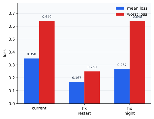
In the graph, when restart_delay_batch is corrected, both the average loss and the worst loss fall together. By contrast, when only night_shift_batch is corrected, the average loss falls but the red bar, that is, the largest loss, remains unchanged. So the core point reinforced by this graph is that did the average decrease? and did the largest weakness decrease? must be read separately.
If the same output is turned into operational judgment, it becomes even more direct.
| Example scene | Interpretation that is easy to make if only the result is read quickly | Better interpretation |
|---|---|---|
night_shift_batch and stabilized_batch | Since both are only slightly wrong, the priority gap is not very large | Both are mild correction candidates, but night_shift_batch may need to be adjusted before stabilized_batch |
restart_delay_batch | Since it is included in the average anyway, overall adjustment will solve it naturally | Read restart_delay_batch as the signal that represents the input region where the model is currently especially weak, because it pulls up the loss the most |
Looking only at mean_loss | It is easy to feel that as long as the overall loss falls, that is enough | Read that even if the average falls, you still have to check which sample remains the worst case before the real correction direction becomes clear |
Is a Model Always Good If the Loss Is Small
Readers can easily feel that once the loss number becomes smaller, everything is solved. But the following must also be remembered.
- when reading loss, you should check not only whether the number itself became smaller, but also whether it fell only on the training data or remained stable on the validation data as well
- even with the same small loss, if you do not distinguish from which data region the value came, overfitting can easily be missed
- if you trust the model only from training loss, overfitting can be missed
In other words, loss is the central standard of learning, but it still has to be read together with the validation split, test set, and metrics seen in Part 4.
This is exactly why deep learning inherits the common machine-learning principles of Part 4 without change.
When Should the Loss-Function View Be Read First
The moment when the loss-function section needs to be brought in is when the explanation the model produced an output is still not enough to make it clear that learning has started.
| Problem scene that appears first | Why the loss-function view is useful first | The next question to pass forward immediately |
|---|---|---|
| An output was produced, but what is wrong is not yet compared numerically | It fixes the standard that turns the gap between prediction and target into a signal that learning can use. | We need to see next why the loss changes by problem type. |
| The metric and the learning standard look mixed together | It separates the human-readable metric from the internal standard by which the model learns. | We must next check which losses are natural in regression and classification. |
| Backpropagation or the optimizer suddenly feels out of place | Because only when loss exists does the explanation of what is being reduced finally close. | We must next see how this loss is passed through each layer. |
| Even among wrong answers, the difference in degree matters | It reveals why how far it is off must be left as a number rather than only right or wrong. | We must next see the interpretive differences among kinds of loss. |
Checklist
- Can you explain what the loss function turns into a number?
- Can you distinguish the role difference between loss and metric?
- Can you explain that the loss function is the rule that turns the gap between prediction and target into one number?
- Can you say why learning has not yet started with output alone, and why a loss number is additionally needed?
- Can you explain that loss is the internal standard by which the model learns, while the metric is the external standard read by people?
- Can you explain that learning is the process of changing parameters in the direction that reduces the loss?
- Can you say that a reduced loss does not automatically guarantee generalization?
- When an output was produced but the explanation is still missing what standard the model learns by, can you think of the loss-function view first?
- Do you know the flow that differences among loss types and backpropagation are passed to the next section and next chapter?
Sources and References
- Ian Goodfellow, Yoshua Bengio, Aaron Courville,
Deep Learning, MIT Press, 2016, date checked: 2026-06-29. https://www.deeplearningbook.org/ - Christopher M. Bishop,
Pattern Recognition and Machine Learning, Springer, 2006, date checked: 2026-07-19. https://link.springer.com/book/9780387310732