P5-4.2 Loss By Problem Type
Section ID:
P5-4.2Version:v2026.07.26
In P5-4.1, we looked at the loss function as the standard that turns how far the model's current output differs from the target into a number. The next question then appears naturally.
Do we use the same loss function for every problem?
The answer is no.
The loss function changes by problem type, because regression, classification, and generation each have a different shape of wrongness.
When the standards for reading loss differently by problem type start to get mixed together again, return to the loss function, mean squared error, MSE, and cross-entropy entries in the concept glossary.
The Question Where Problem Type Changes the Loss
- Why do regression and classification use different loss standards?
- How should a problem of matching numbers be read differently from a problem of matching probabilities?
- In generation problems, why does
how plausibly the next token was predictedconnect directly to loss? - What differences does the choice of loss function make in the direction of learning?
This section explains why the loss changes by problem, rather than showing many formulas. The derivatives of loss and the flow of learning updates reconnect in P5-5.1 and P5-5.2. In other words, this section first closes why what counts as wrong changes depending on the problem type.
Standards for Output Interpretation and Loss Choice
- You can distinguish the viewpoint of loss in regression, classification, and generation problems.
- You can explain that regression centers on the size of numeric error, classification on confidence in the correct class, and generation on the probability of the next token.
- You can understand that the loss function must be designed to match the shape of wrongness in the problem.
- You can explain which predictions should be corrected more strongly first by problem type.
Why Does the Loss Change by Problem
If the problem type changes, then the meaning of the phrase it is wrong also changes.
For example:
- in predicting batch energy use, what matters is
how far away was it? - in classifying inspection states, what matters is
how much confidence was placed on the correct class? - in generating operational guidance text, what matters is
how plausibly the next word was predicted
In other words, the loss function is not merely a mathematical formula. It is the rule that decides what should count as wrong in this problem.
If that is reduced into one large flow, it becomes the following.
flowchart TD
  A["problem type"]
  B["what counts as error?"]
  C["choose loss"]

  A --> B
  B --> C
The key point of this diagram is that the problem structure has to be examined before the model.
If the same flow is divided again through the standard what is being read as wrong?, it becomes the following.
flowchart TD
  A["Problem type"]
  B["Regression"]
  C["Classification"]
  D["Generation"]
  E["How far from the target number?"]
  F["How confident is the true class?"]
  G["How probable is the next true token?"]

  A --> B
  A --> C
  A --> D
  B --> E
  C --> F
  D --> G
The result to confirm first in this diagram is that when the problem type changes, what branches first is not the name of the loss formula, but what kind of wrongness is being turned into a number.
What Matters in Regression
Regression is usually the problem of predicting a continuous number.
- batch energy use
- pressure stabilization time
- hourly cooling-water demand
- equipment transfer distance
In these problems, what matters is how far it moved away from the correct number.
In other words, regression loss is designed in the direction of gathering the size of the error into a number.
It is enough to understand it as follows.
- if it is only slightly wrong, the loss is small
- if it is very wrong, the loss is large
Representative examples are viewpoints such as mean squared error (MSE) or mean absolute error (MAE).
What Matters in Classification
Classification is a problem where the correct class is fixed.
- immediate shutdown / continue monitoring
- normal / fine scratch
- remeasurement needed / automatic pass
Here, simple right-or-wrong still matters, but learning needs more detailed information than that.
For example, whether the model:
- gave probability 0.51 to the correct class
- or gave probability 0.99 to the correct class
can both count as correct in the end, but from the viewpoint of learning the difference is clear.
In other words, classification loss is designed in the direction of reading more sensitively how high was the confidence on the correct class? or how confidently did it move toward the wrong class?
That is why cross-entropy appears so often as a representative loss.
What Matters in Generation
A generation problem resembles classification but is still different. Especially in the context of LLMs, the model usually does not learn by matching the whole sentence at once, but by predicting the next token repeatedly.
In other words, generation learning can often be read through the following structure.
- look at the context so far
- place probabilities over candidate next tokens
- learn in the direction of assigning high probability to the actual correct token
Because of this, generation problems also often use a probabilistic loss close to classification. In practice and in textbooks, the cross-entropy or negative log-likelihood (NLL) of the correct token at each position is usually calculated, and then summed or averaged across the whole sequence and across the whole batch to form the objective. The difference is that this is not one binary judgment, but something repeated across a long sequence.
It is enough to understand it like this.
The loss of a generative model is not the loss of memorizing a whole sentence at once. It is the loss built by accumulating how well the next token was predicted at each position.
Comparing Regression and Classification
Even though the same word wrong is used, regression and classification are read in completely different ways.
| Problem type | Output form | Core way of reading wrongness |
|---|---|---|
| Regression | Continuous value | How far did it move away from the correct number? |
| Classification | Class probability | How much confidence was placed on the correct class? |
| Generation | Probability distribution over next tokens | How plausibly was the correct token predicted? |
Once this table is understood, it becomes clear that the loss function is not merely an implementation choice. It reflects the structure of the problem.
If the same content is extended to what becomes blurry if the wrong loss perspective is used, it becomes clearer still.
| Problem type | What the loss must read well | What becomes blurry if read through another problem type |
|---|---|---|
| Regression | The size of numeric error | If it is read like class probability, the feel of actual distance weakens. |
| Classification | Confidence in the correct class and confidence in the wrong class | If only number difference is examined, it becomes difficult to punish confidently wrong strongly enough. |
| Generation | Probability of the correct token at each position | If it is read like one simple right-or-wrong table, the accumulated sequence-wide error becomes blurry. |
In other words, choosing a loss function is, before anything else, the act of deciding what kind of wrongness has to be read most sensitively in this problem, more than choosing a formula name.
This becomes easier if you think that even the horizontal axis of the graph changes. Regression first looks at distance from the correct number, classification at the probability assigned to the correct class, and generation at the probability assigned to the correct token across many positions.
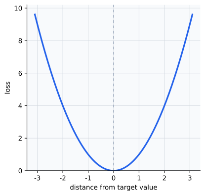
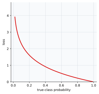
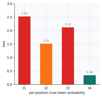
So rather than immediately comparing the sizes of loss numbers across types, you first have to read which prediction is worse inside the same problem type. As these three graphs show, when the problem type changes, the axis that the loss reads changes with it.
Cases and Examples
Case 1. Regression
Suppose we estimate the total energy use of one mixed batch. In this scene, what people first look at is how far is it from the correct usage?
- actual usage: 5.0kWh
- prediction 1: 4.9kWh
- prediction 2: 3.5kWh
Here, prediction 1 is much less wrong. People also easily feel intuitively that 4.9kWh is fairly close, while 3.5kWh is far off. In a regression problem, the important standard is not only whether it is correct or wrong, but how far it moved away. So it is natural for the loss to give a smaller number to prediction 1 and a larger warning signal to prediction 2. Only with that difference can an energy-prediction model distinguish between a model that needs only a small correction and a model that needs to be reconsidered more broadly.
| Standard a person is likely to look at first | Standard reread from the viewpoint of regression loss |
|---|---|
| Both are not the correct answer, so both are just wrong | First look at how far each one moved away from the correct number |
| Look only at whether the usage range was roughly right | Leave behind more strongly in number form whether the error was 0.1kWh or 1.5kWh |
| Judge the degree of deviation only in words | Turn it into a loss number so that many samples can be compared by the same standard |
So the result to confirm in this case is whether the prediction that moved farther away from the correct answer actually receives a larger loss.
| Misreading a person is likely to make first | Why it is less good | Better reading |
|---|---|---|
Group 4.9kWh and 3.5kWh together as simply wrong answers | Then a prediction that needs only a little correction and a prediction that needs a large correction are not distinguished | In regression, read the error distance first and see the farther prediction as the priority for correction |
Read regression loss as if it were the probability of belonging to the correct range | It leads to misunderstanding a continuous-value problem as if it were a classification problem | Read regression loss as a distance-based error signal, not a probability |
Case 2. Classification
Suppose a surface-inspection model reads one frame. People usually first look at did it get it right?, but in actual operation, how confidently did it get it right? also matters. Let the correct class be fine scratch.
- prediction 1: fine scratch 0.55, normal 0.45
- prediction 2: fine scratch 0.95, normal 0.05
Both predict the correct answer, but from the viewpoint of learning, it is natural to read prediction 2 as much better. People can easily feel that both are similar because fine scratch ranks first in both, but in a classification problem it matters greatly how strongly did it push the correct answer to first place? In an inspection system that directly decides automatic pass or not, if got it right but was almost confused and got it right confidently are treated as the same thing, the next learning direction becomes blurry. For example, when an automatic-confirmation threshold is used, 0.55 may be sent to human review while 0.95 may be sent directly to the rework queue. So classification loss has to look more finely at the probability distribution than at a simple answer sheet.
| Standard a person is likely to look at first | Standard reread from the viewpoint of classification loss |
|---|---|
Since both rank fine scratch first, they are almost the same | Also look at how strongly the correct answer was pushed into first place |
| Feel that one answer-sheet cell is enough | Regard 0.55 and 0.95 as very different learning signals |
| Think the confidence gap matters only later in operational policy | See that the confidence gap already affects the update size from the loss stage onward |
So the result to confirm in this case is whether, even though both are correct answers, the lower-confidence prediction actually leaves behind a larger loss.
| Output scene | Less bad misreading | More dangerous misreading | Better reading |
|---|---|---|---|
fine scratch 0.55, normal 0.45 | Read it as barely correct, but still unstable | End it with it is correct, so there is nothing more to look at | Read that even if it is correct, a low-confidence answer still leaves a larger loss and additional learning signal |
fine scratch 0.95, normal 0.05 | Read it as a better prediction | Mistake 0.95 itself for the operational policy | Read that high confidence in the correct answer means a smaller loss, but the policy is still decided separately |
Case 3. Generation
Imagine a model generating operational guidance text or work-instruction text and choosing the next token. People often feel that it is enough to check only whether the correct word was ranked first, but in actual learning it matters how strongly the correct token was pushed upward. Suppose the correct next token is confirm.
- prediction 1: confirm 0.40, remeasure 0.35, hold 0.25
- prediction 2: confirm 0.85, remeasure 0.10, hold 0.05
Here too, it is natural for generation loss to read prediction 2 as better. People can easily feel that the two are similar because both place confirm first, but in actual generation the probability given to the correct token changes the size of the next update. For example, in building summary sentences or operational guidance tokens, if this difference accumulates across positions, it becomes a difference in the quality of the whole sentence. In other words, generation loss reads more finely not did it rank the right answer first?, but how strongly did it push the correct token?
| Standard a person is likely to look at first | Standard reread from the viewpoint of generation loss |
|---|---|
If both rank confirm first, they are similar | Also look at how much probability was given to the correct token |
| It feels enough to check only whether one position was correct | See that this probability difference accumulates across many positions of the sequence |
| It is easy to feel that only the final sentence quality matters | Learning accumulates next-token loss at each position and carries that into whole-sentence quality |
So the result to confirm in this case is whether, even when both rank the correct token first, the prediction that gave the correct token a stronger probability actually leads to a smaller loss and a clearer update in learning.
In other words, generation loss is tightly connected to how much probability was given to the correct next token.
| Output scene | Less bad misreading | More dangerous misreading | Better reading |
|---|---|---|---|
confirm 0.40, remeasure 0.35, hold 0.25 | Read that the correct token was ranked first, but still weakly | Think it is enough just because the top rank was correct | Read that generation loss cares not only about the top rank, but also about how weak the correct-token probability still is |
confirm 0.85, remeasure 0.10, hold 0.05 | Read it as a better prediction | Conclude that the quality of the whole sentence is already fully guaranteed | Read that the loss at one position is small, but sentence quality becomes stable only when this kind of judgment accumulates across many positions |
When the three cases are placed side by side, the difference among loss functions by problem type does not stop at the formula names are different.
| Problem type | Judgment people are likely to make first | What the loss reveals more finely | Prediction that should be corrected more strongly first |
|---|---|---|---|
| Regression | The prediction farther from the actual value is worse | It spreads how much larger the error distance is into a clearer loss number | the 3.5kWh prediction |
| Classification | If both are correct, they can look similar | It further separates how much confidence was placed on the correct class | the fine scratch 0.55 prediction |
| Generation | If both place the correct token first, they can look similar | It shows how the probability gap for the correct token accumulates into loss across positions | the confirm 0.40 prediction |
The result readers should first hold from this table is that regression filters again through distance, classification through confidence in the correct class, and generation through the probability of the correct token at each position.
The reason machine learning and deep learning curricula explain loss by problem type separately is that understanding only the model structure is not enough to understand learning.
Even with the same neural network:
- if the final output is a continuous value, it has to be read through regression loss,
- if the final output is class probability, it has to be read through classification loss,
- if the final output is a token distribution, it has to be read through generation loss.
In other words, the internal structure of a neural network and the loss function are not separate topics. The meaning of the final output directly determines how the loss should be understood with it.
This flow becomes especially important later when looking at LLMs. You need to understand that the learning loss of an LLM does not directly measure whole sentence quality, but is built by accumulating next-token prediction loss across many positions. This explanation also connects immediately to expressions frequently seen in outside literature, such as next-token cross-entropy, token-level NLL, and sequence loss.
Practice and Exercise
The goal of this exercise is to confirm with very small numbers how the viewpoint for reading loss differs between regression and classification. This time, instead of looking at only one value, we first fix the comparison standards: error distance in regression and probability of the correct class in classification.
This time generation is added as well, so that even inside predictions that place the correct answer first, we can also check why the loss still reads a more fine-grained difference.
Input:
- 2 regression predictions and the target
- 2 probabilities for the correct class in classification
- 2 probabilities for the correct token in generation
Output:
- 2 regression losses based on error
- 2 classification losses based on probability
- 2 generation losses based on position-wise probability
- comparison results showing which prediction is worse inside each problem
Problem situation:
- regression, classification, and generation all use loss, but they should not be read through the same standard of
badness, because the way they turn wrongness into a number is different
Concepts to confirm:
- regression loss is read through the value difference, classification loss through the size of the probability assigned to the correct class
- generation loss is read through the probability assigned to the correct token at each position
- even inside the same problem, it must still be possible to distinguish the less bad prediction from the more bad prediction
- it is important that when the problem type changes, the loss calculation changes with it
Input:
Use the regression predictions and target values, the classification correct-class probabilities, and the generation correct-token probabilities organized above.
Before looking at the table, it is useful first to predict which one will become the larger loss.
| Comparison scene | Larger loss to predict first | Reason to expect it |
|---|---|---|
Regression: pred_close=4.7 vs pred_far=3.8 | pred_far | Because it is farther away from the correct answer 5.0. |
Classification: scratch_prob=0.80 vs scratch_prob=0.35 | the 0.35 side | Because it gave lower probability to the correct class. |
Generation: confirm_token_prob=0.75 vs confirm_token_prob=0.30 | the 0.30 side | Because even for the same correct token, the position that assigned lower probability will create a larger loss in the next update. |
The purpose of this table is not to compare the numbers of regression, classification, and generation loss directly with one another. It is to hold that the standards for deciding which prediction is worse are different inside each problem.
If the same comparison is organized through the loss results, it can be read as follows.
| Problem type | Less bad prediction | More bad prediction | Loss result | Core point to read now |
|---|---|---|---|---|
| Regression | pred_close=4.7 | pred_far=3.8 | 0.09 vs 1.44 | The one farther from the correct number receives the larger loss. |
| Classification | scratch_prob=0.80 | scratch_prob=0.35 | 0.223 vs 1.05 | The one with lower probability on the correct class receives the larger loss. |
| Generation | confirm_token_prob=0.75 | confirm_token_prob=0.30 | 0.288 vs 1.204 | The one with weaker probability on the correct token receives the larger loss. |
The goal here is not to compare the size of the numbers directly between regression and classification. What matters is which prediction is read as worse inside each problem.
- Regression loss looks at the difference in numbers.
- So
pred_far, which is farther away, receives the larger loss. - Classification loss looks at the probability assigned to the correct class.
- So
scratch_prob=0.35, which gave less probability to the correct class, receives the larger loss. - Generation loss looks at the probability assigned to the correct token at each position.
- So even though both ranked the correct token first,
confirm_token_prob=0.30, which gave it weaker probability, receives the larger loss.
If this result is tied again into one line, it becomes the following.
| Problem type | Core standard that separates the worse prediction | Side that received the larger loss in this example |
|---|---|---|
| Regression | Distance from the correct number | pred_far=3.8 |
| Classification | Probability of the correct class | scratch_prob=0.35 |
| Generation | Probability of the correct token | confirm_token_prob=0.30 |
In other words, the meaning of the loss number changes depending on the problem structure.
After reading the output, it is better to connect once more which prediction should be corrected more strongly first.
| Problem type | Prediction that should be corrected more strongly first in this output | Reason for reading it that way | Immediate next judgment |
|---|---|---|---|
| Regression | pred_far=3.8 | Because it is much farther away from the correct answer 5.0, so the error distance is far larger. | Before adjusting the prediction value itself, first look at why the input features and weights missed by so much. |
| Classification | scratch_prob=0.35 | Because the probability given to the correct class is low, so the danger of drifting toward the wrong class is larger. | First check whether it is a sample near the boundary, and why the logit gap became narrow. |
| Generation | confirm_token_prob=0.30 | Because even if the correct token ranks first, the weak confidence can shake later positions as well. | First check whether the earlier context was insufficient, or why the competing token became strong. |
Once this table is read, it becomes clearer that the core of loss by problem type does not end at calculating a number, but also at separating again which prediction should be corrected more strongly first.
From the viewpoint of learning, what has to close here is not the name of the loss formula, but the shape of wrongness. You should be able to say for yourself that in regression it is distance, in classification it is insufficient probability for the correct class, and in generation it is insufficient probability for the correct token at each position that create update priority. Only then can backpropagation and LLM training loss later be read in the same flow.
| Axis to change and reread | Loss difference that becomes clearer | Question to raise now |
|---|---|---|
Move pred_far in regression closer to the correct answer | How quickly the distance-based loss shrinks | In regression, which region is the core error region? |
Raise scratch_prob=0.35 to 0.55 in classification | How much the lack of correct-class confidence is eased | How much does weak confidence near the boundary enlarge the learning signal? |
Look at confirm_token_prob=0.30 repeated across many positions in generation | The structure in which small probability shortages at each position accumulate into sequence-wide loss | Why is LLM loss read not as a whole sentence at once, but as accumulated next-token loss? |
Even when this comparison is tested in Python, the key is not to make the absolute values compete with one another. The example below separates what loss decreases when only one weak prediction is corrected in regression, classification, or generation.
When executed, it becomes the following.
The values to manipulate in this example are energy_prediction, scratch_probability, and token_probability. If the regression prediction is moved closer to the correct answer, only the regression loss decreases. If the correct-class probability is raised, only the classification loss decreases. If the correct-token probability is raised, only the generation loss decreases. So rather than deciding which problem is worse by placing the three numbers on one line, you must first read what changed inside the same problem when the loss decreased.
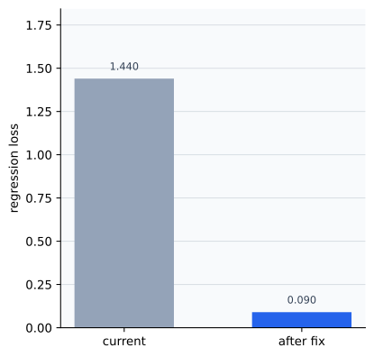
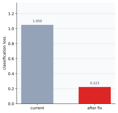
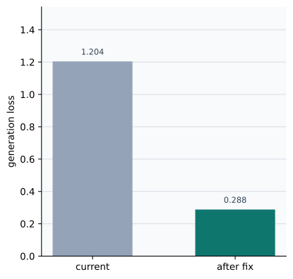
The three graphs do not try to force different problems into one picture. They show only how loss decreases from current -> after adjustment inside each problem. In regression, loss decreases when the prediction is moved closer to the correct answer. In classification, it decreases when the probability of the correct class rises. In generation, it decreases when the probability of the correct token rises. So when reading the graphs, you should first look not at the absolute heights of the three losses against one another, but only at the before-and-after change inside each graph.
One more point needs special care here: the goal is not to compare the absolute values of the three numbers directly.
| Problem type | Less bad misreading | More dangerous misreading | What must be checked first now |
|---|---|---|---|
| Regression | Only see that 0.09 is small, so it seems mostly fine | Compare regression loss 1.44 and classification loss 1.05 directly and conclude which is worse | First look at the difference in distance from the correct answer inside the same problem |
| Classification | Only see that scratch_prob=0.35 is worse | Read a probability-based loss number as if it had the same unit as a regression-error number | Look at how much the probability of the correct class is lacking |
| Generation | Only see that confirm_token_prob=0.30 is worse | Conclude the quality of the whole sentence from one generation-loss number alone | See that the position-wise probability gap accumulates repeatedly |
What Becomes Visible When It Connects All the Way to Generative Models
In a generative model, a classification-like loss is repeated across a long sequence. So an LLM can structurally be read like a very large classification problem repeated once for each next token.
If readers know this connection, then later in Part 5, when words such as token, next-token prediction, cross-entropy, and perplexity appear, they feel less abrupt.
In other words, the explanation of the loss function in Part 5 is also preparation for understanding LLM training in the next Part.
When Should Loss Be Read by Problem Type
After understanding the general role of the loss function, the loss has to be separated out according to what counts as wrong in this problem.
| Problem scene that appears first | Loss viewpoint to think of first | Reason |
|---|---|---|
| A continuous number is predicted | Regression loss | Because what matters is how far it moved away from the correct number. |
| The correct class must be identified | Classification loss | Because what matters is how strongly the correct class is supported. |
| The next token is generated one by one | Generation loss | Because what matters is how strongly the correct token is pushed at each position. |
| The confidence gap matters even among the same wrong answers | Probability-based classification/generation loss | Because the difference in distribution has to be read more finely than a simple answer sheet. |
Checklist
- Can you explain why regression, classification, and generation use different loss standards?
- Can you say that when the problem type changes, the shape of
wrongnesschanges as well? - Can you explain that the loss function changes depending on the problem type?
- Can you explain that regression is read through numeric error, classification through the probability of the correct class, and generation through the probability of the next token?
- Can you say that even with the same neural-network structure, if the meaning of the output changes, the loss standard changes too?
- When confidence matters in classification or generation more than a simple answer sheet, can you bring back the probability-based interpretation of loss?
- Can you explain why next-token prediction connects directly to loss structure by reading generation loss through the viewpoint of repeated classification?
- Do you understand the flow that after this section comes the chapter on backpropagation, where we examine how the loss is passed to earlier layers?
Sources and References
- Ian Goodfellow, Yoshua Bengio, Aaron Courville,
Deep Learning, MIT Press, 2016, date checked: 2026-06-29. https://www.deeplearningbook.org/ - Christopher M. Bishop,
Pattern Recognition and Machine Learning, Springer, 2006, date checked: 2026-07-19. https://link.springer.com/book/9780387310732