P5-5.1 How Does Loss Become a Gradient Signal
Section ID:
P5-5.1Version:v2026.07.26
In Chapter P5-4, we saw that the loss function turns the mismatch between the current output and the target into a number. But the loss number alone still cannot change the parameters.
Loss tells us how wrong it is, but which parameter should move in which direction and by how much has to be computed separately.
The signal needed here is the gradient. A gradient is the value that shows how sensitively the loss responds to a specific parameter. Backpropagation is the procedure that starts from the loss and computes that gradient from the later calculations back toward the earlier ones.
When this starts to blur together again with the computation graph or the optimizer in later sections, return to the backpropagation, gradient, and chain rule entries in the concept glossary and separate the computational roles first.
Fix these three sentences first in this section.
- Loss turns how wrong the current output is into a number.
- The gradient computes what direction and strength each parameter has in relation to the loss.
- The optimizer receives that gradient and performs the actual parameter update.
The Question of How Loss Becomes a Gradient
- Why can't the loss number alone update the parameters directly?
- What additional information does the gradient provide?
- How is backpropagation the procedure that computes gradients from the loss?
- How does automatic differentiation make this computation possible in code?
- How is gradient computation different from the optimizer update?
The viewpoint of unfolding complex computational relationships into nodes and connections continues in P5-5.2, and the role of the optimizer, which turns gradients into actual parameter movement, reconnects in P5-7.1 and P5-7.2. Here, we first close the point that learning can continue only when the loss number is turned into a per-parameter gradient signal.
Standards for Direction and Size Signals
- You can distinguish loss, gradient, and optimizer update.
- You can explain the gradient as
the signal that shows how sensitive the loss is to a specific parameter. - You can explain backpropagation as
the procedure that starts from the loss and moves backward through the earlier calculations to compute gradients. - You can explain automatic differentiation as
the technique that automatically organizes gradient computation by using the forward-pass record. - You can confirm with a small example that loss magnitude and gradient direction are not the same thing.
Why Isn't Loss an Update Yet
Loss is one number. For example, even if the loss of a model is 4.0, that number alone cannot answer the following questions.
In actual deep-learning implementations, instead of differentiating one per-sample loss as it is, many cases differentiate an objective/cost built from a batch average or sum plus regularization terms. But at the stage where the reader first needs to grasp the role of the gradient, it is enough to understand that the core starting point of the whole objective is still the mismatch signal created by the loss.
- Which parameter is more strongly connected to this loss?
- Should that parameter be increased or decreased?
- Is a small movement enough, or does it need a large movement?
So learning needs a step after loss. The loss has to be unpacked again into a signal for each parameter.
| Step | Question it asks | Result |
|---|---|---|
| Loss computation | How far is the current output from the target? | Loss number |
| Gradient computation | What direction and strength does each parameter have in relation to the loss? | Per-parameter gradients |
| Optimizer update | How much should the model actually move using the computed gradients? | New parameter values |
The important point in this table is that gradient computation and update are different. The gradient is the signal for how it should move, and the optimizer decides the actual movement rule by using that signal.
What Does the Gradient Tell Us
The gradient tells us how sensitive the loss is to a parameter. Look at the following simple expression.
Even if the loss \(L\) is large here, that fact alone does not tell us whether risk_weight should be increased or decreased. If the predicted score is below the target, increasing risk_weight may be needed. If the predicted score is above the target, decreasing it may be needed.
The gradient leaves that difference behind through sign and size.
| What we read from the gradient | Meaning |
|---|---|
| Sign | When the parameter is increased slightly, does the loss increase or decrease? |
| Magnitude | How sensitive is the loss to that parameter? |
In other words, loss tells us the size of the wrongness, and the gradient tells us the sensitivity signal for each parameter. The actual update usually moves not in the direction where the loss increases, but in the opposite direction. So if the gradient is positive, decreasing the parameter is the direction that lowers the loss, and if the gradient is negative, increasing the parameter is the direction that lowers the loss.
Where Does Backpropagation Fit
Neural networks are structures where many calculations are connected.
flowchart TD
  A["forward pass<br/>input -> hidden -> output"]
  B["loss computed at output"]
  C["backward pass<br/>output -> hidden -> input-side weights"]

  A --> B
  B --> C
The forward pass starts from the input and computes the output and the loss. Backpropagation starts from the loss and moves backward through the earlier calculations to compute gradients.
The first result to confirm in this flow is that the forward pass and backpropagation answer different questions. First there is the flow that computes the output and the loss. Then there is the gradient computation that starts from the loss and travels back toward the earlier parameters.
Why Compute from Back to Front
The output layer is most directly connected to the loss.
- there is the final output
- there is the target value
- and the loss is computed by comparing the two
So the easiest thing to know first is how does the loss respond to the final output? After that, we use the fact that the final output depended on the previous layer's values and parameters, and send the influence backward one step at a time.
The forward pass and backpropagation are not the same statement with opposite directions. The two flows ask different questions.
| Flow | Direction of computation | Question it asks |
|---|---|---|
| Forward pass | Goes from the input to the output and loss | What did it predict now, and how wrong was it? |
| Backward pass | Travels from the loss back to the earlier parameters | What gradient does that error leave on each parameter? |
In other words, backpropagation is computed from back to front because the loss is already at the end of the computation. We have to compute the gradient for the calculation closest to the loss first, then pass that gradient to the earlier calculations so that the update signal reaches the parameters in the earlier layers.
If we draw it very simply, it looks like this.
flowchart TD
  A["forward pass<br/>input -> hidden -> output"]
  B["loss computed at output"]
  C["backward pass<br/>output -> hidden -> input-side weights"]

  A --> B
  B --> C
The key point of this diagram is the order: look at the output error -> compute the gradient of the last calculation -> pass that influence to the earlier calculation -> repeat until the first layer.
Why Does the Chain Rule Appear
Neural networks are structures where functions are stacked over many stages.
For example, in a very simple form, it looks like this.
flowchart LR
    x["input x"] --> z["intermediate z"]
    z --> a["intermediate a"]
    a --> y["output y"]
    y --> loss["loss"]
The loss does not depend directly on the original input or the earlier parameters. It is connected indirectly through many intermediate values. In this structure, we have to connect how a change in one stage affects the next stage. That is where the chain rule appears.
It is enough to understand it like this.
If a later result depends on an earlier value, then the influence has to be propagated by multiplying the dependency stage by stage.
The question to grasp before the formula is this.
If the output of this layer became the input of the next layer, then doesn't the error created later have to share some gradient with the earlier layer too?
The chain rule is the rule that makes this intuition mathematically possible. Backpropagation is the procedure that efficiently applies the chain rule to the deep functional structure of a neural network and turns the loss into a per-parameter gradient signal.
Why Do We Need to Understand Automatic Differentiation Too
In modern deep learning, users do not expand every derivative formula by hand. Frameworks such as PyTorch, TensorFlow, and JAX record the forward computation process, then follow it backward from the loss and automatically organize the gradient computation.
This technique is automatic differentiation.
Automatic differentiation does not create gradients by magic. It records which value was created by which operation during the forward pass, then applies the derivative rule of each operation in reverse order to compute the gradients.
The level needed in this section is roughly the following.
| Category | What we need to know in this section | What we do not go deeply into here |
|---|---|---|
| Backpropagation | The procedure that starts from the loss and computes the gradients of the earlier parameters | A rigorous matrix-derivative derivation for the whole deep network |
| Automatic differentiation | The fact that the framework automatically organizes gradient computation by using the forward-pass record | The memory management, optimizations, and internal implementation of the autodiff engine |
| Computation graph | A way to understand what computation is recorded and followed | Details of graph-engine implementation |
So automatic differentiation is not a topic you can ignore. It is a concept needed to understand why backpropagation runs in actual code. But the general theory of automatic differentiation and the internal implementation of frameworks are not the central scope of P5-5.1.
Cases and Examples
Case 1. The Update Direction Can Differ Even When There Is Loss
Think of a small model that predicts a restart-block score. The input is pressure_unrecovered, the parameter is risk_weight, and the target is target_block_score.
People tend to look first at whether the loss is large or small. But at the learning stage, the size of the loss alone is not enough. We also have to distinguish between the case where the prediction is below the target and risk_weight needs to increase, and the case where the prediction is above the target and risk_weight needs to decrease.
For example, let pressure_unrecovered = 2.0 and target_block_score = 5.0. If risk_weight = 1.5, the predicted score is 3.0. If risk_weight = 3.2, the predicted score is 6.4. Loss appears in both cases, but what learning has to do is the opposite. In the first case, the score is too small, so risk_weight has to increase. In the second case, the score is too large, so risk_weight has to decrease.
flowchart TD
    start["Compute the predicted score"] --> compare["Compare it with the target score"]
    compare --> loss["Loss: how far off is it?"]
    compare --> grad["Gradient: increase or decrease, and how sensitive?"]
    grad --> update["Use it to decide the next parameter adjustment"]
There is one result to hold first in this small scene. Loss only leaves behind the fact that it is wrong, while the gradient leaves behind which direction and how strongly it should be corrected.
| Case | Relationship between prediction and target | If you look only at the loss | If you also look at the gradient |
|---|---|---|---|
| Predicted slightly low | Slightly smaller than the target | The error is small | A weak signal to increase risk_weight |
| Predicted far too low | Much smaller than the target | The error is large | A strong signal to increase risk_weight |
| Predicted too high | Larger than the target | There is an error | A signal to decrease risk_weight |
The difference becomes even clearer if the same table is split into the question loss answers and the question the gradient answers.
| Value you are looking at now | Question it answers immediately | Blank that still remains |
|---|---|---|
| Loss | How far off is it? | Who should move in which direction? |
| Gradient | Which parameter should increase or decrease? | How far will the optimizer actually move it? |
The result to confirm in this case is that if loss is the stage that tells us the size of the error, then the gradient is the stage that rewrites that error into direction and strength for each parameter.
Case 2. Why Isn't Fixing Only The Final Score Enough
Real neural networks do not create one score immediately. They first combine many inputs into intermediate representations, then produce the final output. For example, imagine first combining temperature warning, pressure warning, and vibration warning into an overall risk signal, then creating the final stop score from that.
When the final score is wrong, it is easy to feel that looking only at the last layer should be enough. But the final score already depends on the overall risk signal made by the earlier layers, so we may need to correct how strongly the earlier layers combined those inputs as well.
This is exactly where the intuition of backpropagation matters.
- if the final output is wrong, it is not only the last connection that has responsibility
- the earlier representation that created that last connection also has responsibility
- and the still earlier weights that created that representation also receive gradients
In other words, backpropagation is not fix only the final score. It is the structure of divide the gradient of the output error step by step all the way to the earlier layers. So the result to confirm in this case is whether gradients of different sizes and directions actually attach not only to the last layer but also to the weights in the earlier layers.
If we compress the two cases together again, the first flow to hold in this section is the following.
flowchart TD
    A[Prediction is too low] --> B[Need to raise the score]
    B --> C[Gradient marks increase direction]

    D[Prediction is too high] --> E[Need to lower the score]
    E --> F[Gradient marks decrease direction]

    G[Final score is wrong] --> H[Backward responsibility starts]
    H --> I[Last layer gets a signal]
    I --> J[Earlier layers also receive responsibility]
This diagram is there to gather together, at once, the directional sense from Case 1, the score is too small / too large, and the structure from Case 2, the gradient is passed all the way to the earlier layers. The key here is the flow look at the loss -> a direction appears -> the gradient is passed from back to front.
When the two cases are placed side by side, backpropagation is not a procedure that only says the loss is large. It is the procedure that rewrites who has to be corrected, and by how much and in what way for each parameter.
| Scene | Interpretation that is easy to leave behind if you look only at the loss | What gradient computation makes clearer |
|---|---|---|
| Correcting one score | It feels like if the prediction is small, increase it, and if it is large, decrease it | It leaves behind not only the direction but also the correction strength for each parameter |
| Final score after many inputs | It feels like you should look only at the last output and fix only the last layer | It distributes gradients to the intermediate layer and the earlier layers too |
The result the reader should hold first in this table is that the key point is not we know the loss, but we turn the loss back into a per-parameter gradient signal.
Practice and Example
The goal of this example is not to implement the whole of backpropagation. We use a very small expression to check how the loss number and the gradient signal differ. Instead of looking at only one case, we run together a case where the block score is too small and a case where the block score is too large so we can also see how the sign of the gradient changes.
Input:
- pressure unrecovered level
pressure_unrecovered - target block score
target_block_score - current risk weight
risk_weight
Output:
- predicted block score
- loss
- gradient with respect to
risk_weight - correction direction indicated by the gradient
Problem scene:
- if you look only at the formula, the gradient still feels abstract, so it is better to see directly how the direction changes when the block score is too small and when it is too large
- even under the same direction, we also need to see whether a larger error produces a larger gradient magnitude
Concepts to confirm:
- loss is always 0 or greater, so it does not directly contain direction information
- by looking at the sign of the gradient, we can interpret which direction the parameter should move to reduce the loss
- the magnitude of the gradient shows how sensitive the loss is to that parameter
Before looking at the code, it is helpful to predict what kind of signal each case will produce.
| Case | Comparison to predict first | Why that is the expected result |
|---|---|---|
slightly_under_block_signal | increase_risk_weight, but probably weak in strength | It is only a little below the target, so the direction is to increase it, but the correction may not need to be large. |
too_weak_block_signal | increase_risk_weight, and probably stronger in strength | Even though the direction is the same, it falls farther short of the target, so the gradient magnitude may become larger. |
too_strong_block_signal | decrease_risk_weight | Since it is above the target, the signal should point in the opposite direction. |
The purpose of this table is to practice reading direction and strength separately, not to memorize formulas.
The value to change directly is risk_weight. If you place it near 2.5, the prediction gets closer to the target. If you make it smaller or larger, you can check how the sign and magnitude of the gradient change.
Read the output like this.
This output has to be read by separating it into predicted score -> loss -> gradient.
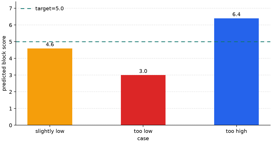
The first graph shows the predicted block score for each case. The target is 5.0. The first two cases are below the target, and the last case is above it.
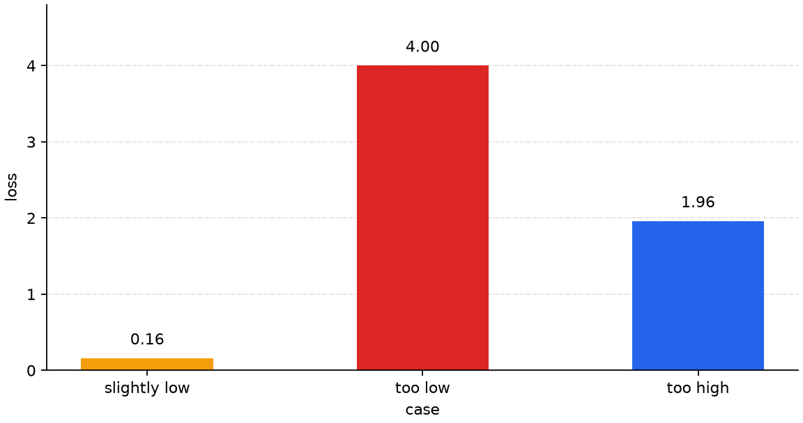
The second graph is the loss. Loss shows the size of the error, but it does not directly show the direction. For example, the mere fact that there is a loss does not tell us whether risk_weight should increase or decrease.
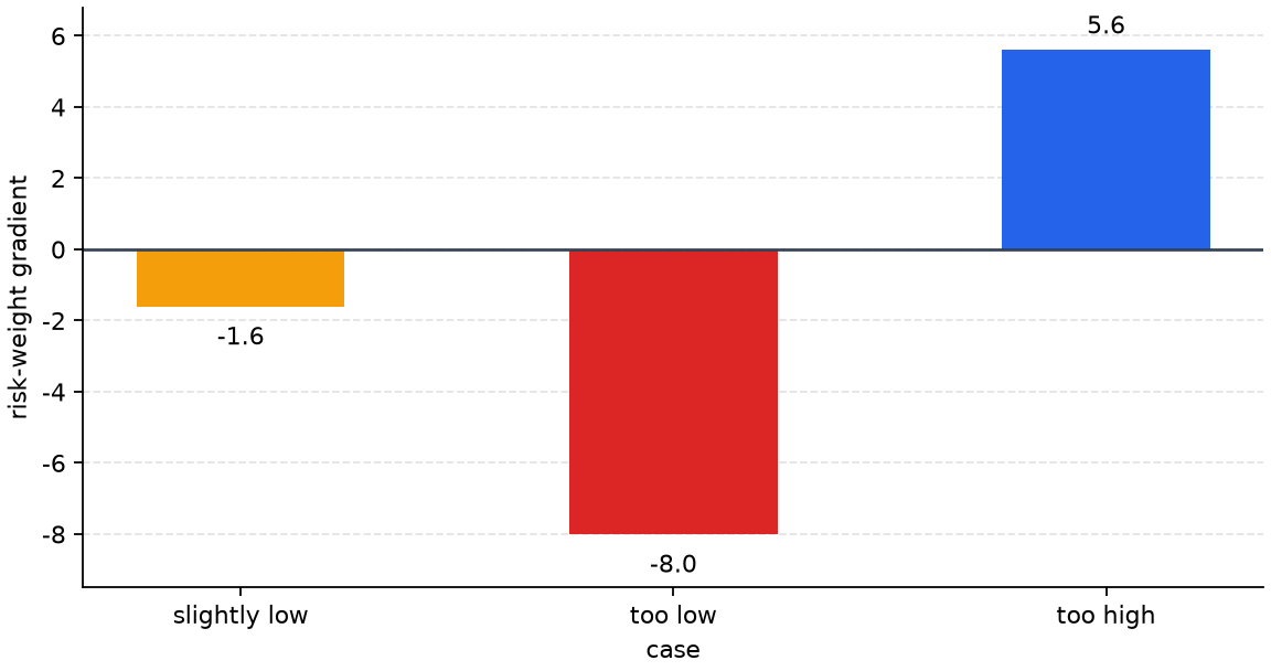
The direction appears in the third graph. A negative gradient is read as the direction to increase risk_weight, and a positive gradient is read as the direction to decrease it. So the key change in this example is not the loss number, but the per-parameter gradient signal.
When the three cases are gathered together again, it becomes clear that we have to read sign and size together.
| Case | What appears in the loss | What appears in the gradient | Core point to read now |
|---|---|---|---|
slightly_under_block_signal | The error is small | A weak increase signal | It falls only a little short of the target, so it should increase, but this is close to fine adjustment. |
too_weak_block_signal | The error is large | A strong increase signal | Even under the same increase direction, it falls much farther short, so the gradient magnitude grows larger. |
too_strong_block_signal | There is an error | A decrease signal | The direction itself flips, so risk_weight has to decrease. |
- When the block score is too small, the gradient becomes negative and gives a direction signal to increase
risk_weight. - When the block score is too large, the gradient becomes positive and gives a direction signal to decrease
risk_weight. - Even inside the same direction, when the error is larger, the gradient magnitude grows and becomes a stronger correction signal.
The sentence that must remain from this example is the following.
Loss turns the wrongness into a number, and the gradient rewrites that wrongness into direction and strength for each parameter.
If the result is split again by the standards of loss and gradient, the difference becomes even sharper.
| Difference shown in the execution result | Interpretation that is easy to leave behind if you look only at the loss | Interpretation that changes when you also look at the gradient |
|---|---|---|
slightly_under_block_signal and too_weak_block_signal both have a block score that is too small | It is easy to read only that both need a larger risk weight | It reads which one receives the stronger increase signal even under the same direction |
too_weak_block_signal and too_strong_block_signal both have loss | It is easy to feel that similar corrections are needed because both have error | The direction itself splits: one increases, the other decreases |
| Only one loss number stands out first | It is easy to feel that knowing the error size is enough | It reads that actual updates need an additional per-parameter gradient signal |
Once this table is read, it becomes clearer again that the core of backpropagation is not the loss was computed, but the loss was rewritten into direction and size for each parameter.
What Becomes Harder in Multi-Layer Neural Networks
The example above was simple because it had only one parameter. In a multi-layer neural network, the situation becomes difficult immediately.
- the output arrives through many layers
- each layer has many parameters
- and the value of each layer becomes the input to the next layer
So we need a procedure that redistributes the influence of the loss back across each layer and parameter. Backpropagation computes these gradients efficiently by starting from the loss and traveling backward through the earlier calculations. Automatic differentiation lets the framework organize that computation automatically based on the execution record.
It is enough to remember it like this.
As the layers get deeper, it becomes difficult to write the gradients by hand, but backpropagation systematically passes the computation from back to front.
In the history of backpropagation there were earlier precursors and contributions, but in the context of neural-network learning, the widely known turning point is the 1986 paper by Rumelhart, Hinton, and Williams. That work helped show broadly that multi-layer neural networks could learn useful internal representations.
More broadly, earlier work such as Paul Werbos's 1974 doctoral thesis is also often mentioned. Here, it is enough to remember the following.
- there were earlier mathematical and optimization ideas
- and in the mid-1980s it became widely known as a neural-network learning procedure and marked a major turning point
From the curriculum viewpoint too, backpropagation is an important section. If P5-4.1 and P5-4.2 explained why we use a loss function, we now need to understand how that loss is passed to the parameters of each layer. The reason is simple.
- even if there is a loss function
- if we do not know how that loss is connected to each layer
- actual learning updates become impossible
In other words, backpropagation is the gradient-computation procedure that makes it possible to say deep learning is actually trained.
In the next section, P5-5.2, we unfold this execution record as a computation graph. Once you look at the computation graph, it becomes clearer what intermediate values are created during the forward pass and along what path the gradient travels back during the backward pass.
When Do We Read from the Viewpoint of Gradient Computation
| Problem scene that appears first | Why the viewpoint of gradient computation is needed | The next question to hand off immediately |
|---|---|---|
| You know the loss, but do not know which parameter to change | The loss has to be unpacked into direction and strength for each parameter | In a complex computation, how do we track that signal? |
| It feels like if the loss is large, we should always update by a large amount | Loss size and update direction are not the same information | How will the optimizer use this gradient as a step size? |
It looks like magic that the framework computes gradients with .backward() | We need to know that automatic differentiation uses the forward-pass record | What does the computation graph record? |
Checklist
- Can you explain that parameters are not updated immediately just because the loss was computed?
- Can you explain that the gradient is a signal of direction and strength for each parameter?
- Can you say that backpropagation is the procedure that starts from the loss and moves backward through the earlier calculations to compute the gradient?
- Can you explain that automatic differentiation automatically organizes gradient computation by using the forward-pass computation record?
- Can you distinguish gradient computation from optimizer update?
- Do you understand that the reason for looking at the computation graph in the next section is
to track complex gradient computation?
Sources and Further Reading
- David E. Rumelhart, Geoffrey E. Hinton, Ronald J. Williams,
Learning representations by back-propagating errors, Nature, 1986, accessed 2026-07-19. https://doi.org/10.1038/323533a0 - Paul J. Werbos,
Beyond Regression: New Tools for Prediction and Analysis in the Behavioral Sciences, Harvard University doctoral thesis, 1974, accessed 2026-07-19. https://cir.nii.ac.jp/crid/1572261550254843264?lang=en - Ian Goodfellow, Yoshua Bengio, Aaron Courville,
Deep Learning, MIT Press, 2016, accessed 2026-06-29. https://www.deeplearningbook.org/