P5-5.2 Computation Graphs¶

Section ID: P5-5.2 Version: v2026.07.23

In P5-5.1, we explained that loss is not itself an update, but has to be unpacked again into a per-parameter gradient signal. Once that much is understood, the next question remains.

When there are many layers and the computation becomes complex, what computation does the framework record so that it can automatically calculate the gradient?

The viewpoint that answers this question is the computation graph and automatic differentiation.

A computation graph is a representation that unfolds a model's computation into nodes and edges so that we can see where values are created in the forward pass and along what path automatic differentiation sends gradients back during backward.

When you need to unfold the computational relationships into a smaller reading again, use the computation graph entry in the concept glossary as the anchor.

The Question Of How Computation Graphs Remember Differentiation¶

• What does a computation graph represent?
• Why do we look at deep-learning computations as graphs?
• How are the forward pass and backward pass read on the graph?
• What relationship does it have with automatic differentiation?

This section does not teach graph theory itself. Instead, it explains why automatic differentiation becomes possible only when deep-learning computations are recorded like a graph.

From the point of view of Part 5, getting to this point already closes the responsibility needed to understand gradient computation. Rather than adding a separate supplemental study of backpropagation mathematics, it fits the current flow of the book better to build intuition here for loss to gradient, the chain rule, the computation graph, and automatic differentiation, and then move to the optimizer sections. So here, rather than reading a new model structure, we read how the structure we already saw is recorded and how gradients are sent back.

Standards For Dependencies And Automatic Differentiation¶

• You can explain a computation graph as a recorded structure that unfolds computational dependencies.
• You can read on the graph that the forward pass is value computation and the backward pass is gradient propagation.
• You can understand that the computation graph breaks complex differentiation into small steps.
• You can explain that automatic differentiation automatically organizes gradient computation by using the computation graph and local derivative rules.
• You can confirm the flow of storing intermediate values and computing gradients with an executable Python example.

What Does A Computation Graph Draw¶

Neural networks are not magic boxes that turn input into the answer all at once. In practice, they are structures where many small operations are connected.

For example:

• receive input \(x\)
• multiply by weight \(w\)
• add bias \(b\)
• pass through an activation function
• compute the loss

If we read this flow only as prose, it quickly becomes complicated. A computation graph is a picture that divides these operations into small stages and connects them.

In other words, a computation graph shows the following two things at the same time.

1. where a value is created
2. how the dependency relationship continues

Why Do We Need To See It As A Graph¶

As formulas become longer, backpropagation often starts to feel abstract. The reason is that we are looking at the whole expression as one large block.

But if we turn it into a computation graph:

• the large formula is broken into small operations
• we can see which node depends on which other node
• and it becomes visible that the gradient also follows the same path in reverse

In other words, a computation graph does not create a new differentiation method. It makes the existing computational flow visible.

It is enough to understand it like this.

A computation graph divides one large formula into small boxes so that forward computes values and backward sends influence back.

Looking At The Smallest Example¶

Consider the following expression.

If we look at this only as a single line, it may not seem complicated. But in a neural network, this kind of structure repeats thousands or tens of thousands of times. That is why the viewpoint of dividing it into nodes of small operations becomes important.

If we draw it very simply, it looks like this.

flowchart TD
  X["x"]
  W["w"]
  M["multiply<br/>wx"]
  B["b"]
  Z["add<br/>z = wx + b"]
  A["ReLU<br/>a"]
  T["target t"]
  L["loss L"]

  X --> M
  W --> M
  M --> Z
  B --> Z
  Z --> A
  A --> L
  T --> L

This figure shows two things.

• in the forward pass, values are computed from left to right
• in the backward pass, gradients start from the loss and travel from right to left

How Do We Read The Forward Pass On The Graph¶

The forward pass is the stage that computes actual numbers at each node of the graph.

For example:

1. the multiply node receives \(w\) and \(x\) and makes \(wx\)
2. the add node adds \(b\) to that result and makes \(z\)
3. the ReLU node receives \(z\) and makes \(a\)
4. the loss node compares \(a\) and the target \(t\) and makes the loss

In other words, the forward pass is the process of following the graph and filling in intermediate values.

The reason storing these intermediate values matters is that the backward pass needs those exact values again.

How Do We Read The Backward Pass On The Graph¶

The backward pass is the stage that starts from the loss node and moves backward while computing how much each earlier node contributed to the loss.

For example:

• first look at how sensitive the loss is to \(a\)
• then look at how sensitive \(a\) is to \(z\)
• then divide again how sensitive \(z\) is to \(w\), \(x\), and \(b\)

So the graph decomposes the following question step by step.

If this value changes a little, how much does the final loss change?

This decomposition is exactly how the chain rule becomes an actual computational procedure.

How Does A Computation Graph Make The Chain Rule Easier¶

In P5-5.1, the chain rule was explained as the rule that connects influence stage by stage. The computation graph makes those stages visible.

For example, if the loss \(L\) depends on \(a\), \(a\) depends on \(z\), and \(z\) depends on \(w\), then instead of memorizing

all at once, we can read in sequence:

• how sensitive \(L\) is to \(a\)
• how sensitive \(a\) is to \(z\)
• how sensitive \(z\) is to \(w\)

It is enough to remember it like this.

A computation graph does not treat differentiation as one giant formula, but divides it into small local rules at each node.

Its Relationship To Automatic Differentiation¶

When we use modern deep-learning frameworks, there are many cases where we do not write every backpropagation formula by hand. Tools such as PyTorch, TensorFlow, and JAX automatically compute gradients by using the computation graph.

The important point here is the following.

Automatic differentiation does not create gradients by magic. It is the procedure that systematically applies local derivative rules along the computation graph.

So if we want to understand automatic differentiation, it is natural to understand the computation graph first.

This much is enough.

• forward: compute values and remember them
• backward: compute gradients by following the remembered flow
• automatic differentiation: the framework organizes these two stages for us

flowchart TD
  A["forward pass<br/>input -> hidden -> output"]
  B["loss computed at output"]
  C["backward pass<br/>output -> hidden -> input-side weights"]

  A --> B
  B --> C

Cases And Examples¶

Case 1. If We Look Only At The Final Block Score, The Computation Path Disappears¶

Think about a very small computation that reads the level of unrecovered pressure and produces a restart-block score. Operators tend to look first only at the final block score and judge it is high, it is low, or it differs from the target. But from the viewpoint of the computation graph, before the final score we unfold the intermediate computations that produced it.

For example, suppose the input signal pressure_signal is multiplied by the risk weight risk_weight to produce weighted_pressure, then a baseline offset base_block_bias is added to make block_logit, and after passing through ReLU we get block_activation. The final loss then computes how far this output is from the target block score target_block_score. If we read this only as a one-line formula, it sounds like nothing more than we computed the loss. But on the computation graph, each node becomes visible separately.

What beginners most easily miss here is treating one final score and the full path that made that score as if they were the same thing. For example, if the block score is 0.8, a person may immediately interpret that as the risk was judged high. But the computation graph asks one more question. Did that 0.8 happen because pressure_signal itself was large, because risk_weight amplified it strongly, because base_block_bias had already created a high baseline, or because the pre-ReLU block_logit was positive and therefore passed through? We have to split those possibilities first.

In other words, the final block score is the result, but what matters more on the computation graph is the path the result passed through. In pressure_signal -> weighted_pressure, the input and the weight meet. In weighted_pressure -> block_logit, a baseline offset is added. In block_logit -> block_activation, ReLU decides whether the value passes through or is blocked. Once we separate these stages, it becomes visible that the same block score 0.8 could arise for completely different reasons. In one case the input signal itself was large. In another case the input was not large, but the weight and bias pushed the score upward.

This distinction is needed because when we read gradients later, we have to trace node by node what has how much responsibility. If we look only at the final score, we are left only with the fact that the value was large, while the operations that made it large disappear. If we unfold it as a computation graph instead, we can separately read which intermediate value became the material for later computation, where the sign or magnitude of the value changed, and which parameter actually affected the later output.

flowchart TD
    score["final block score"]
    score --> question["score alone is not enough"]
    question --> path["reopen the path:<br/>pressure_signal -> weighted_pressure<br/>-> block_logit -> block_activation"]
    path --> read1["which node made the score larger?"]
    path --> read2["which node will receive gradient later?"]
    read1 --> result["read the score together with its computational path"]
    read2 --> result

So the result to confirm in this case is not the final block score itself, but whether the intermediate outputs along weighted_pressure -> block_logit -> block_activation -> loss are actually split into visible stages. The computation graph has to create that separation so we can later read how far the gradient returns.

Case 2. The Loss Is Large, But The Gradient Does Not Reach The Earlier Part¶

Even in the same computational network, the interpretation of backpropagation changes depending on whether block_logit is positive or negative. If block_logit > 0, ReLU passes the value through, so the gradient that starts from the loss can continue through block_activation -> block_logit -> risk_weight, base_block_bias. But if block_logit <= 0, the forward output is cut to 0, and in backward the gradient is not passed to the earlier side before ReLU.

The point that especially confuses beginners here is automatically connecting the fact that the loss is large with the expectation that the earlier parameters must also be corrected a lot. For example, suppose the target block score is 1.0, but the actual block_activation is 0 and the loss becomes large. A person may naturally think, If it is this wrong, shouldn't the earlierrisk_weightbe corrected strongly too? But the computation graph does not look only at the size of the loss. It separately checks how far the gradient that starts from the loss can actually travel back through the nodes.

It becomes clearer if we unfold the case where the ReLU gate is closed step by step. First, in the forward pass, if block_logit is computed as 0 or less, the block_activation after ReLU becomes 0. At this point the output can still be far from the target, so the loss can be large. But when we come back in backward, ReLU sends a gradient of 0 for paths where the input was 0 or less. Then the signal that started from the loss exists up to block_activation, but it no longer continues through block_logit to risk_weight and base_block_bias. In other words, there can be a case where the degree of wrongness is large, yet that wrongness does not lead to earlier-parameter correction along this path.

If we restate this at a beginner-friendly level, it becomes this. The fact that the output missed badly and the fact that we can travel back along this path and correct it are separate matters. Loss shows the error of the result, but the gradient shows whether the path inside the computation network is actually open for that error to travel back. If the ReLU gate is closed, the path can be cut even when the loss is large. So when reading a computation graph, right after asking how badly is it wrong?, we also need to ask separately how far does that wrongness propagate as responsibility?

flowchart TD
    loss["loss is large"]
    loss --> gate["check block_logit at the ReLU gate"]
    gate --> open["block_logit > 0"]
    gate --> closed["block_logit <= 0"]
    open --> live["backward path stays alive"]
    live --> update["risk_weight and bias can be updated"]
    closed --> stop["gradient becomes 0 at ReLU"]
    stop --> noupdate["front parameters do not update through this path"]

So the important learning point in this case is not large loss = large update, but large loss + a live backward path is what leads to earlier-parameter correction. Even with the same loss number, if the sign of the value before ReLU changes, the backward interpretation changes completely. When block_logit > 0, responsibility travels back to risk_weight and base_block_bias. When block_logit <= 0, the gradient can stop there. The tool that lets us separate this difference visually is the computation graph.

In this scene, people tend to look only at the loss number and think, the side with the larger loss should be corrected more strongly. But the computation graph does not read it that way. Even if the loss is large, if the path is cut, the earlier parameters are not updated through that path. So the computation-graph viewpoint separates how wrong is it from how far does responsibility travel back.

So there are two results to confirm in this case. First, in forward, look at which node creates which value. Second, in backward, look at whether the gradient that starts from the loss is still alive when it reaches the nodes before ReLU and the parameters. Only when these two questions are separated does the computation graph become not just a picture of computational order, but a tool for reading backpropagation.

When the two cases are placed together, it becomes clearer why the computation graph is needed.

flowchart TD
    A[Prediction is too low] --> B[Need to raise the score]
    B --> C[Gradient marks increase direction]

    D[Prediction is too high] --> E[Need to lower the score]
    E --> F[Gradient marks decrease direction]

    G[Final score is wrong] --> H[Backward responsibility starts]
    H --> I[Last layer gets a signal]
    I --> J[Earlier layers also receive responsibility]

Practice And Example¶

The goal of this example is not to use an automatic-differentiation library, but to directly confirm in a very small expression what intermediate values are created in forward and what gradients are computed in backward. The role of this example is not to write code that trains the model well, but to build the reading standard for following each node of the computation graph by hand.

So the code here takes on only three roles.

• it reveals side by side the forward values and backward gradients along the same computation graph
• it stops us from reading the loss is large and the gradient path is alive as if they were the same statement
• it compresses what an automatic-differentiation framework does internally into a tiny computational network

Input:

• pressure unrecovered level pressure_signal
• pressure risk weight risk_weight
• baseline offset base_block_bias
• target block score target_block_score

Output:

• forward intermediate values weighted_pressure, block_logit, block_activation, loss
• backward gradients d_loss_d_activation, d_loss_d_logit, d_loss_d_weighted_pressure, d_loss_d_weight, d_loss_d_bias
• the connection showing which intermediate value is reused in which gradient computation
• the difference in backward between the case where the ReLU gate is open and the case where it is closed

Problem scene:

• because backpropagation starts from the final loss and traces intermediate values backward, seeing the forward values and backward values together helps understanding
• even with the same formula, if the sign of the pre-ReLU value block_logit changes, the gradient flow can be cut, so we need a comparison

Concepts to confirm:

• the backward gradients in backpropagation are computed by reusing the forward intermediate values
• if we print the intermediate values and gradients together for each stage, it becomes easier to track the computational connection
• for nodes such as ReLU, whether backward is passed on depends on the sign information from forward

The especially important point here is that the correct answer of the example is not one loss number. The correct answer of this example is reading node by node what value was created and at which point the gradient stayed alive or was cut.

Input:

Use the two cases summarized above: pressure_signal, risk_weight, base_block_bias, and target_block_score.

Before looking at the code, it is helpful to predict in which case the gradient will travel farther.

This comparison matters especially on the computation graph because whether the gate is open or closed in forward also changes the backward path.

flowchart TD
  subgraph OPEN["case A: block_gate_open<br/>block_logit = 2.5 > 0"]
    direction TD
    subgraph OPEN_F["forward values"]
      direction LR
      OW["weighted_pressure<br/>3.0"]
      OZ["+ bias<br/>block_logit 2.5"]
      OR["ReLU open<br/>activation 2.5"]
      OL["loss<br/>2.25"]

      OW --> OZ --> OR --> OL
    end

    subgraph OPEN_B["backward signals"]
      direction RL
      OA["dL/da<br/>-3.0"]
      OZG["dL/dz<br/>-3.0"]
      OWG["dL/dw = -6.0<br/>dL/db = -3.0"]

      OA --> OZG --> OWG
    end

    OL --> OA
  end

  subgraph CLOSED["case B: block_gate_closed<br/>block_logit = -0.3 <= 0"]
    direction TD
    subgraph CLOSED_F["forward values"]
      direction LR
      CW["weighted_pressure<br/>0.2"]
      CZ["+ bias<br/>block_logit -0.3"]
      CR["ReLU closed<br/>activation 0.0"]
      CL["loss<br/>16.0"]

      CW --> CZ --> CR --> CL
    end

    subgraph CLOSED_B["backward signals"]
      direction RL
      CA["dL/da<br/>-8.0"]
      CZG["dL/dz<br/>0.0"]
      CWG["dL/dw = 0.0<br/>dL/db = 0.0"]
      CSTOP["blocked at ReLU<br/>front parameters are not updated by this path"]

      CA -. "ReLU derivative 0" .-> CZG
      CZG -.-> CWG
      CZG -.-> CSTOP
    end

    CL --> CA
  end

  OPEN ~~~ CLOSED

  classDef open fill:#f0fdf4,stroke:#16a34a,color:#166534
  classDef closed fill:#fef2f2,stroke:#ef4444,color:#991b1b
  classDef loss fill:#fff7ed,stroke:#f97316,color:#9a3412
  classDef zero fill:#f8fafc,stroke:#94a3b8,color:#475569

  class OW,OZ,OR,OA,OZG,OWG open
  class CW,CZ,CR closed
  class OL,CL loss
  class CA,CZG,CWG,CSTOP zero

This diagram makes us separate is the loss larger? from does the gradient actually reach the earlier parameters? before looking at the output numbers. block_gate_closed has the larger loss, but on the computation graph the path is cut before ReLU, so the gradient does not reach risk_weight and base_block_bias.

 1
 2
 3
 4
 5
 6
 7
 8
 9
10
11
12
13
14
15
16
17
18
19
20
21
22
23
24
25
26
27
28
29
30
31
32
33
34
35
36
37
38
39
40
41
42
43
44
45
46
47
48
49
50
51
52
53
54
55
56
57
58
59
60
61
62
63
64
65
66
67
68
69
70
71
72
73
74
75
76
77

# This example traces whether gradients pass back to earlier weight and bias nodes when a ReLU gate is open or closed.
def relu(value):
    return max(0.0, value)

cases = [
    {"name": "block_gate_open", "pressure_signal": 2.0, "risk_weight": 1.5, "base_block_bias": -0.5, "target_block_score": 4.0},
    {"name": "block_gate_closed", "pressure_signal": 2.0, "risk_weight": 0.1, "base_block_bias": -0.5, "target_block_score": 4.0},
]

for case in cases:
    pressure_signal = case["pressure_signal"]
    risk_weight = case["risk_weight"]
    base_block_bias = case["base_block_bias"]
    target_block_score = case["target_block_score"]

    # forward
    weighted_pressure = risk_weight * pressure_signal
    block_logit = weighted_pressure + base_block_bias
    block_activation = relu(block_logit)
    loss = (block_activation - target_block_score) ** 2

    # backward
    d_loss_d_activation = 2 * (block_activation - target_block_score)
    d_activation_d_logit = 1.0 if block_logit > 0 else 0.0
    d_loss_d_logit = d_loss_d_activation * d_activation_d_logit
    d_logit_d_weighted_pressure = 1.0
    d_loss_d_weighted_pressure = d_loss_d_logit * d_logit_d_weighted_pressure
    d_logit_d_weight = pressure_signal
    d_logit_d_bias = 1.0
    d_loss_d_weight = d_loss_d_logit * d_logit_d_weight
    d_loss_d_bias = d_loss_d_logit * d_logit_d_bias

    node_trace = [
        {
            "node": "weighted_pressure = risk_weight * pressure_signal",
            "forward_value": round(weighted_pressure, 3),
            "backward_signal": round(d_loss_d_weighted_pressure, 3),
            "read_as": "gradient that returned to the weighted_pressure output",
        },
        {
            "node": "block_logit = weighted_pressure + base_block_bias",
            "forward_value": round(block_logit, 3),
            "backward_signal": round(d_loss_d_logit, 3),
            "read_as": "gradient that stays alive or is cut before ReLU",
        },
        {
            "node": "block_activation = ReLU(block_logit)",
            "forward_value": round(block_activation, 3),
            "backward_signal": round(d_loss_d_activation, 3),
            "read_as": "the output node that the loss looks at directly",
        },
        {
            "node": "loss = (block_activation - target_block_score) ** 2",
            "forward_value": round(loss, 3),
            "backward_signal": "start",
            "read_as": "the loss node where backward starts",
        },
    ]

    print(f"[{case['name']}]")
    print("forward:", {
        "weighted_pressure": round(weighted_pressure, 3),
        "block_logit": round(block_logit, 3),
        "block_activation": round(block_activation, 3),
        "loss": round(loss, 3),
    })
    print("backward:", {
        "d_loss_d_activation": round(d_loss_d_activation, 3),
        "d_loss_d_logit": round(d_loss_d_logit, 3),
        "d_loss_d_weighted_pressure": round(d_loss_d_weighted_pressure, 3),
        "d_loss_d_weight": round(d_loss_d_weight, 3),
        "d_loss_d_bias": round(d_loss_d_bias, 3),
    })
    print("node_trace:")
    for row in node_trace:
        print(" ", row)
    print("---")

In the output, do not look at the loss number only. Read it in the order forward summary -> backward summary -> node_trace. The first two lines summarize the values, and node_trace is the core of this example. That is exactly where we can follow each node of the computation graph again and reread where a value was created and where a gradient stayed alive or was cut.

 1
 2
 3
 4
 5
 6
 7
 8
 9
10
11
12
13
14
15
16
17
18

[block_gate_open]
forward: {'weighted_pressure': 3.0, 'block_logit': 2.5, 'block_activation': 2.5, 'loss': 2.25}
backward: {'d_loss_d_activation': -3.0, 'd_loss_d_logit': -3.0, 'd_loss_d_weighted_pressure': -3.0, 'd_loss_d_weight': -6.0, 'd_loss_d_bias': -3.0}
node_trace:
  {'node': 'weighted_pressure = risk_weight * pressure_signal', 'forward_value': 3.0, 'backward_signal': -3.0, 'read_as': 'gradient that returned to the weighted_pressure output'}
  {'node': 'block_logit = weighted_pressure + base_block_bias', 'forward_value': 2.5, 'backward_signal': -3.0, 'read_as': 'gradient that stays alive or is cut before ReLU'}
  {'node': 'block_activation = ReLU(block_logit)', 'forward_value': 2.5, 'backward_signal': -3.0, 'read_as': 'the output node that the loss looks at directly'}
  {'node': 'loss = (block_activation - target_block_score) ** 2', 'forward_value': 2.25, 'backward_signal': 'start', 'read_as': 'the loss node where backward starts'}
---
[block_gate_closed]
forward: {'weighted_pressure': 0.2, 'block_logit': -0.3, 'block_activation': 0.0, 'loss': 16.0}
backward: {'d_loss_d_activation': -8.0, 'd_loss_d_logit': -0.0, 'd_loss_d_weighted_pressure': -0.0, 'd_loss_d_weight': -0.0, 'd_loss_d_bias': -0.0}
node_trace:
  {'node': 'weighted_pressure = risk_weight * pressure_signal', 'forward_value': 0.2, 'backward_signal': -0.0, 'read_as': 'gradient that returned to the weighted_pressure output'}
  {'node': 'block_logit = weighted_pressure + base_block_bias', 'forward_value': -0.3, 'backward_signal': -0.0, 'read_as': 'gradient that stays alive or is cut before ReLU'}
  {'node': 'block_activation = ReLU(block_logit)', 'forward_value': 0.0, 'backward_signal': -8.0, 'read_as': 'the output node that the loss looks at directly'}
  {'node': 'loss = (block_activation - target_block_score) ** 2', 'forward_value': 16.0, 'backward_signal': 'start', 'read_as': 'the loss node where backward starts'}
---

You can read this output like a table, but if we separate it into graphs, the difference between the size of the forward values and whether the backward gradient survives splits more clearly.

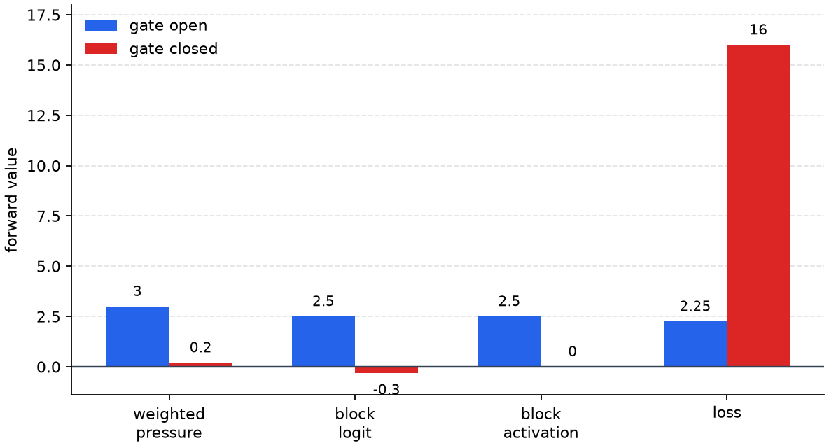
On the forward graph, what appears first is that the loss of block_gate_closed is much larger. But if we look only at this graph, it is easy to misread it as the loss is larger, so the earlier part will also be updated more strongly. That is why we need to split the same example again into a backward graph.

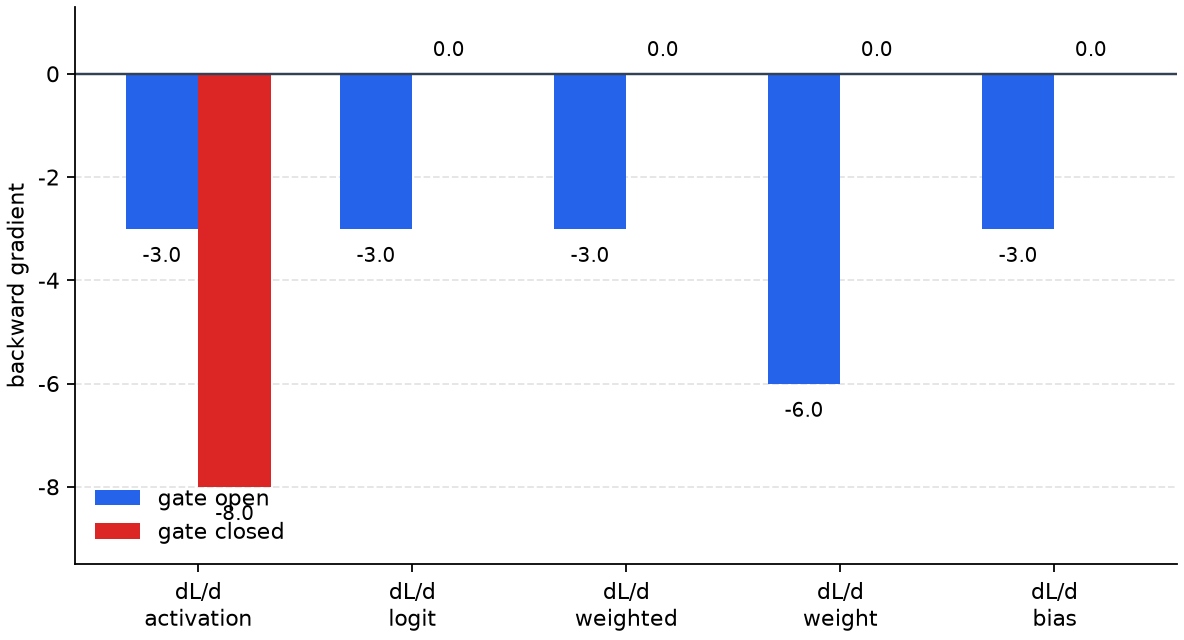
On the backward graph, the contrast appears the other way. In block_gate_open, dL/d_logit, dL/d_weight, and dL/d_bias are all alive. In block_gate_closed, even though dL/d_activation is large, the gradients after the earlier side of ReLU are cut to 0. In other words, when reading a computation graph as a graph, we have to separate the loss bars and the gradient bars.

The important points of this example are the following.

• in forward, intermediate values are created step by step
• in backward, the change that starts from the final loss is decomposed all the way to the earlier parameters
• each node can participate in gradient computation as long as it knows only its local relation to the nodes before and after it
• if we read along node_trace, it becomes clearer that this computation-graph example is not a loss-computation example, but a node-by-node reading example

In other words, the role of this Python example is not to make the reader memorize one more backpropagation formula, but to let the reader hold again, in one block of output, the nodes, intermediate values, local rules, and path blocking explained in the computation-graph section.

Here, reading the two cases side by side makes the computation-graph intuition clearer.

In other words, the computation graph does not only show is the loss large? It also lets us read at which node the gradient flow is alive and where it is cut.

Even when reading the output numbers, we have to separate loss size from gradient path.

In other words, the computation graph breaks a large problem into small local computations.

The computation-graph viewpoint is not only an educational picture. It is a practical entrance to understanding modern deep-learning automatic differentiation and learning systems.

As deep learning spread widely, neural-network structures became more and more complex, and expanding the full derivatives by hand stopped being practical. At that point, the viewpoint of reading operations as a graph and combining local derivative rules became a much more practical explanation.

From the curriculum viewpoint, the result to confirm in this section is whether the backpropagation intuition from P5-5.1 is now read more systematically, not as simple formula memorization, but as the connection of computational blocks and local derivative rules.

• intuition for backpropagation alone can still leave the computational flow blurry
• before learning the optimizer, we need a clearer view of where the gradient comes from
• and later structures such as CNNs, RNNs, and attention are in fact more naturally read as connections among computational blocks

In other words, the computation graph can be seen as a common reading tool for all of Part 5.

When Do We Raise It To A Computation Graph¶

The time to bring out the computation-graph section is when the intuition of backpropagation is there, but the computation has so many stages that where values are created and where gradients return starts to blur.

Checklist¶

• Can you explain how the computation graph unfolds the flow of the forward pass and the backward pass?
• Can you read one large formula as a relationship among small computational blocks?
• Can you explain that the computation graph is a representation that unfolds computational dependencies?
• Can you explain that the forward pass is the stage that computes values along the graph, and the backward pass is the stage that sends back the gradient that started from the loss along the graph?
• Can you say why the intermediate values made in forward are needed again in backward?
• When reading the computation graph, can you trace how the gradient is passed by connecting the local rules of each operation block instead of depending on one giant derivative formula?
• When automatic differentiation starts to feel like magic, can you bring out the viewpoint that it is a procedure organized along the graph by local derivative rules?
• Do you understand that after this section, the flow moves to the optimizer that uses the gradient for actual updates, and to the distinction between learning and inference?

Sources And Further Reading¶

• Ian Goodfellow, Yoshua Bengio, Aaron Courville, Deep Learning, MIT Press, 2016, accessed 2026-06-29. https://www.deeplearningbook.org/
• Christopher M. Bishop, Pattern Recognition and Machine Learning, Springer, 2006, accessed 2026-07-19. https://link.springer.com/book/9780387310732
• Andrej Karpathy, micrograd, GitHub, accessed 2026-06-29. https://github.com/karpathy/micrograd