P5-6.4 Training Mode And Evaluation Mode¶

Section ID: P5-6.4 Version: v2026.07.20

In P5-6.3, we separated learning and model execution (inference) into the time when parameters change and the time when they are used without changing. If we go one step further here, the next question appears.

If the parameters are not changing, do the computational rules also always have to be completely the same?

The answer is not always. Some layers can behave differently in the training-time computational state and the evaluation-time computational state even while using the same parameters. This difference has to be understood clearly so that dropout, batch normalization, validation, test, and deployment (inference serving) do not get mixed together.

Training mode is the computational environment that prepares parameter updates, and evaluation mode is the computational environment that stably measures or uses the current model.

When the distinction between modes starts to blur again with the explanation of dropout or batch normalization, return to the training mode and evaluation mode entries in the concept glossary.

The Question That Requires Training And Evaluation Modes¶

• Why do training mode and evaluation mode split?
• Which layers, rather than all layers, are sensitive to the mode difference?
• Why do dropout and batch normalization behave differently by mode?
• Why is evaluation mode important for validation and test?

This section focuses on distinguishing which computational rules are more appropriate during learning and which are more appropriate during evaluation, even for the same model. In other words, after separating learning and inference, here we close why training mode and evaluation mode are needed even inside a region that uses the same parameters.

At the same time, it is also clear which question we will not widen immediately in this section. The larger meaning of dropout and regularization themselves is treated again in detail in P5-8.1 and P5-8.2, and where the optimizer enters this training flow reconnects again in P5-7.1 and P5-7.2.

Standards For Training-Only Behavior And Execution Behavior¶

• You can explain training mode and evaluation mode as two states where the computational rules differ.
• You can say why dropout and batch normalization are sensitive to the mode difference.
• You can explain why evaluation mode may be needed in validation and deployment.
• You can confirm the mode difference intuitively with an executable Python example.

Why Does The Same Model Need Modes¶

Readers often imagine the model as one fixed function. If the input is the same, they expect it to always compute in the same way and always produce the same result.

But in deep learning, some layers may deliberately inject noise or depend on batch statistics in order to help learning happen better. These layers help during learning, but during evaluation or service execution they can instead create instability.

In other words, mode separation is not just library syntax. It serves the following purposes.

• during learning, allow computations that help generalization
• during evaluation, make results comparable and reproducible more stably

What Does Training Mode Mean¶

Usually, it is enough to read training mode like this.

• it is inside a learning procedure aimed at reducing loss
• after the forward pass, loss computation and backpropagation can continue
• some layers operate in a special way to help learning

In other words, training mode does not mean only the moment when optimizer.step() is called. It means the state in which the model is using learning-time computational rules.

What Does Evaluation Mode Mean¶

Evaluation mode is usually needed in the following situations.

• when measuring performance on a validation set
• when checking final performance on a test set
• when handling real user input in a deployed service

At that time, the key point is to reveal with less fluctuation how well the model does in its current state. So we have to reduce the stochastic fluctuation or batch dependence used during learning, and compute in a more fixed way.

It is enough to understand it like this.

Evaluation mode is the time for measuring how well the model does now, and training mode is the time for changing it to do better.

If we compress this difference down to only the computational rules, it becomes the following.

flowchart TD
  I["Same model input"]

  subgraph T["Training mode"]
    T1["Dropout stays stochastic"]
    T2["Batch statistics are used"]
    T3["Loss and parameter update continue"]
  end

  subgraph E["Evaluation mode"]
    E1["Dropout is turned off"]
    E2["Running statistics are used"]
    E3["Stable measurement or serving output"]
  end

  I --> T1
  T1 --> T2
  T2 --> T3

  I --> E1
  E1 --> E2
  E2 --> E3

The first result to confirm in this diagram is that even for the same model input, training mode separates its computational rules toward allowing fluctuation to prepare updates, while evaluation mode separates them toward stable measurement and service output.

Which Layers Are Sensitive To The Mode Difference¶

Not all layers are sensitive to the mode difference. For example, ordinary linear layers or convolution layers, given the same input and the same parameters, perform broadly the same computation.

But for the following layers, we have to read their behavior during training and during evaluation separately first.

In other words, the mode difference is needed because some layers deliberately operate differently in order to help learning.

Why Is Dropout Different During Training And Evaluation¶

Dropout is a technique that randomly cuts off some node outputs during learning so the model does not rely too heavily on one specific path.

It is enough to understand it like this.

During learning, some connections are deliberately made to rest, so the model does not depend only on one or two signals.

But if we also randomly cut nodes during evaluation every time, the result fluctuates too much. Then it becomes hard to measure stably how well the current model actually performs.

So in evaluation mode, the random removal of dropout is stopped, and the learned network is used in a fixed form.

Why Does Batch Normalization Need A Mode Difference¶

Batch normalization is a layer that adjusts the activation distribution using the mean and variance of each batch. During learning, it is natural to use the current batch statistics, but during evaluation the situation changes.

Evaluation data:

• may have a small batch size
• may contain only one sample
• and may have a different batch composition every time it is measured

In that case, if we use only the current batch statistics every time, the result can become unstable. So in evaluation mode, it usually uses the running statistics accumulated during learning.

It is enough to remember it like this.

During learning, batch normalization refers to the current batch, and during evaluation it refers more to the average standard accumulated during learning.

Why Must Validation And Test Be In Evaluation Mode¶

Validation data and test data are meant to show how well the current model generalizes. If training mode is still on there, dropout can fluctuate randomly and batch normalization can react sensitively to the batch composition.

As a result:

• even with the same model, the measured values can become less stable
• the score can change depending on the batch composition
• and it can become hard to compare them with the felt performance at deployment time

In other words, validation and test are the time to measure the current model fairly, so evaluation mode matters.

Practice And Example¶

The distinction between modes is checked first at moments such as validation, deployment, or small-batch evaluation where the computational rule can disturb interpretation of the result. Even the same input batch can split into different computational rules in training mode and evaluation mode, so the example below checks the difference through stage-by-stage outputs. If we directly put in lists of numbers as in an earlier version, the result can look like hand-made values, so here we first compute one hidden-layer activation from a small user-session batch and then apply the mode difference of dropout and batch normalization to that value.

Input:

• click count and dwell time by session
• a simple weight and bias for one hidden layer
• dropout rate
• random seeds to reproduce two training-mode executions
• previous training-session batches to use in evaluation mode

Output:

• hidden-layer activations computed from the input features
• activations after dropout
• the reference mean used for normalization
• the simplified output after subtracting the reference mean

Problem scene:

• even for the same input, training mode has to allow fluctuation, while evaluation mode should compute with a stable reference

Concepts to confirm:

• in training mode, some activations are turned off randomly
• batch normalization in training mode can use the current batch standard
• in evaluation mode, dropout is stopped and a fixed reference such as running statistics accumulated during learning is used

Input:

Use the current validation-session batch and previous training-session batches summarized above. Here, the hidden-layer computation multiplies recent click count, dwell time, and error count by weights, adds the bias, and then applies only ReLU, which cuts negative values to 0. To keep the explanation simple, batch normalization here computes only value - reference mean. Real batch normalization also uses variance and trainable scale and shift, but in this example we look only at which mean is used as the reference.

Before looking at the code, it helps to predict which stage is computed from the data, and which stage fluctuates or stays fixed because of the mode.

The purpose of this table is not to guess the exact numbers. It is to hold before the code that in training mode, even the same input can produce different dropout results and different batch references between two runs, while evaluation mode stops that fluctuation and builds a baseline.

  1
  2
  3
  4
  5
  6
  7
  8
  9
 10
 11
 12
 13
 14
 15
 16
 17
 18
 19
 20
 21
 22
 23
 24
 25
 26
 27
 28
 29
 30
 31
 32
 33
 34
 35
 36
 37
 38
 39
 40
 41
 42
 43
 44
 45
 46
 47
 48
 49
 50
 51
 52
 53
 54
 55
 56
 57
 58
 59
 60
 61
 62
 63
 64
 65
 66
 67
 68
 69
 70
 71
 72
 73
 74
 75
 76
 77
 78
 79
 80
 81
 82
 83
 84
 85
 86
 87
 88
 89
 90
 91
 92
 93
 94
 95
 96
 97
 98
 99
100
101
102
103
104
105
106
107
108
109
110
111
112
113
114
115
116
117
118
119
120
121
122
123
124

# This example compares how dropout and the batch reference mean fluctuate or stay fixed in train and eval modes.
from random import Random

validation_sessions = [
    {"id": "S01", "clicks_5m": 3, "dwell_seconds": 42, "error_count": 0},
    {"id": "S02", "clicks_5m": 6, "dwell_seconds": 55, "error_count": 1},
    {"id": "S03", "clicks_5m": 2, "dwell_seconds": 28, "error_count": 0},
    {"id": "S04", "clicks_5m": 7, "dwell_seconds": 70, "error_count": 2},
    {"id": "S05", "clicks_5m": 4, "dwell_seconds": 36, "error_count": 0},
    {"id": "S06", "clicks_5m": 5, "dwell_seconds": 48, "error_count": 1},
    {"id": "S07", "clicks_5m": 1, "dwell_seconds": 24, "error_count": 0},
    {"id": "S08", "clicks_5m": 8, "dwell_seconds": 73, "error_count": 2},
    {"id": "S09", "clicks_5m": 4, "dwell_seconds": 52, "error_count": 1},
    {"id": "S10", "clicks_5m": 6, "dwell_seconds": 61, "error_count": 0},
    {"id": "S11", "clicks_5m": 2, "dwell_seconds": 39, "error_count": 1},
    {"id": "S12", "clicks_5m": 7, "dwell_seconds": 58, "error_count": 2},
]
weights = {"clicks_5m": 0.18, "dwell_seconds": 0.015, "error_count": 0.32}
bias = -0.35
drop_rate = 0.4

def make_prior_batch(rows, dwell_shift, error_shift):
    batch = []
    for row in rows:
        batch.append({
            "clicks_5m": row["clicks_5m"],
            "dwell_seconds": max(12, row["dwell_seconds"] + dwell_shift),
            "error_count": max(0, row["error_count"] + error_shift),
        })
    return batch

prior_session_batches = [
    make_prior_batch(validation_sessions, dwell_shift=-4, error_shift=0),
    make_prior_batch(validation_sessions, dwell_shift=2, error_shift=1),
    make_prior_batch(validation_sessions, dwell_shift=5, error_shift=-1),
]

def hidden_activation(row):
    raw = (
        row["clicks_5m"] * weights["clicks_5m"]
        + row["dwell_seconds"] * weights["dwell_seconds"]
        + row["error_count"] * weights["error_count"]
        + bias
    )
    return round(max(0.0, raw), 3)

def make_dropout_mask(count, seed):
    rng = Random(seed)
    return [1 if rng.random() >= drop_rate else 0 for _ in range(count)]

def apply_dropout(values, mask, drop_rate):
    scale = 1 / (1 - drop_rate)
    result = []
    for value, keep in zip(values, mask):
        if keep == 0:
            result.append(0.0)
        else:
            result.append(round(value * scale, 3))
    return result

def mean(values):
    return round(sum(values) / len(values), 3)

def flatten(rows):
    return [value for row in rows for value in row]

def hidden_batch(batch):
    return [hidden_activation(row) for row in batch]

def center_by_mean(values, reference_mean):
    return [round(value - reference_mean, 3) for value in values]

def summarize(values):
    return {
        "count": len(values),
        "min": round(min(values), 3),
        "max": round(max(values), 3),
        "mean": mean(values),
        "preview": values[:5],
    }

def run_training_mode(name, seed):
    mask = make_dropout_mask(len(activations), seed)
    after_dropout = apply_dropout(activations, mask, drop_rate)
    batch_mean = mean(after_dropout)
    centered_output = center_by_mean(after_dropout, batch_mean)
    return {
        "mode": name,
        "kept": sum(mask),
        "dropped": len(mask) - sum(mask),
        "after_dropout_summary": summarize(after_dropout),
        "reference_mean": batch_mean,
        "centered_preview": centered_output[:5],
    }

def run_evaluation_mode():
    after_dropout = activations[:]
    centered_output = center_by_mean(after_dropout, running_mean)
    return {
        "mode": "eval_run",
        "kept": len(after_dropout),
        "dropped": 0,
        "after_dropout_summary": summarize(after_dropout),
        "reference_mean": running_mean,
        "centered_preview": centered_output[:5],
    }

activations = [hidden_activation(row) for row in validation_sessions]
prior_hidden_batches = [hidden_batch(batch) for batch in prior_session_batches]
running_mean = mean(flatten(prior_hidden_batches))

train_run_1 = run_training_mode("train_run_1", seed=17)
train_run_2 = run_training_mode("train_run_2", seed=29)
eval_run = run_evaluation_mode()

print("validation_session_count =", len(validation_sessions))
print("hidden_activation_summary =", summarize(activations))
print("running_mean_from_prior_batches =", running_mean)
for result in [train_run_1, train_run_2, eval_run]:
    print(result["mode"])
    print("kept/dropped =", result["kept"], "/", result["dropped"])
    print("after_dropout_summary =", result["after_dropout_summary"])
    print("reference_mean =", result["reference_mean"])
    print("centered_preview =", result["centered_preview"])

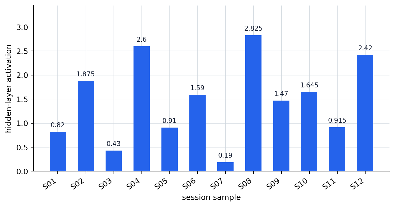
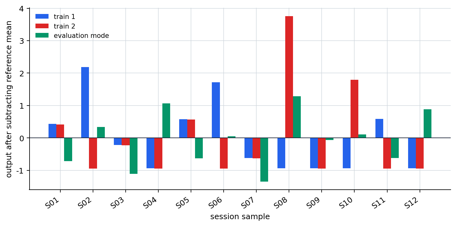
In the output, first confirm that hidden_activation_summary is the summary of the hidden-layer values computed from the input features, then compare kept/dropped, after_dropout_summary, reference_mean, and centered_preview in that order.

 1
 2
 3
 4
 5
 6
 7
 8
 9
10
11
12
13
14
15
16
17
18

validation_session_count = 12
hidden_activation_summary = {'count': 12, 'min': 0.19, 'max': 2.825, 'mean': 1.474, 'preview': [0.82, 1.875, 0.43, 2.6, 0.91]}
running_mean_from_prior_batches = 1.534
train_run_1
kept/dropped = 7 / 5
after_dropout_summary = {'count': 12, 'min': 0.0, 'max': 3.125, 'mean': 0.935, 'preview': [1.367, 3.125, 0.717, 0.0, 1.517]}
reference_mean = 0.935
centered_preview = [0.432, 2.19, -0.218, -0.935, 0.582]
train_run_2
kept/dropped = 6 / 6
after_dropout_summary = {'count': 12, 'min': 0.0, 'max': 4.708, 'mean': 0.947, 'preview': [1.367, 0.0, 0.717, 0.0, 1.517]}
reference_mean = 0.947
centered_preview = [0.42, -0.947, -0.23, -0.947, 0.57]
eval_run
kept/dropped = 12 / 0
after_dropout_summary = {'count': 12, 'min': 0.19, 'max': 2.825, 'mean': 1.474, 'preview': [0.82, 1.875, 0.43, 2.6, 0.91]}
reference_mean = 1.534
centered_preview = [-0.714, 0.341, -1.104, 1.066, -0.624]

This example does not reproduce the whole framework exactly, but the core points to read here are clear.

• the hidden-layer activations are intermediate outputs computed from the input features
• in training mode, even when the same hidden-layer activations are used twice, the number and composition of activations that survive dropout can differ
• if the post-dropout values differ, the reference mean computed from the current batch can also differ
• in evaluation mode, dropout is stopped and a fixed reference such as a running mean accumulated from previous training-session batches is used to make a more stable computational path
• this kind of fluctuation control is exactly why evaluation mode matters in validation, test, and deployment

First, read the same computational rule as a graph. The first graph shows only the result of recent click count, dwell time, and error count in validation-session inputs turning into hidden-layer activations. This stage is not yet the mode difference itself. It is the point where the input data turns into an intermediate representation inside the model.

The next graph shows how the same hidden-layer activations lead to different final output interpretations depending on the mode. train 1 and train 2 are two learning executions with different dropout masks, while eval is the execution computed with dropout off and using the running mean as the reference. If a value is above 0, it means the output is above that reference mean. If it is below 0, it means the output is below that reference mean.

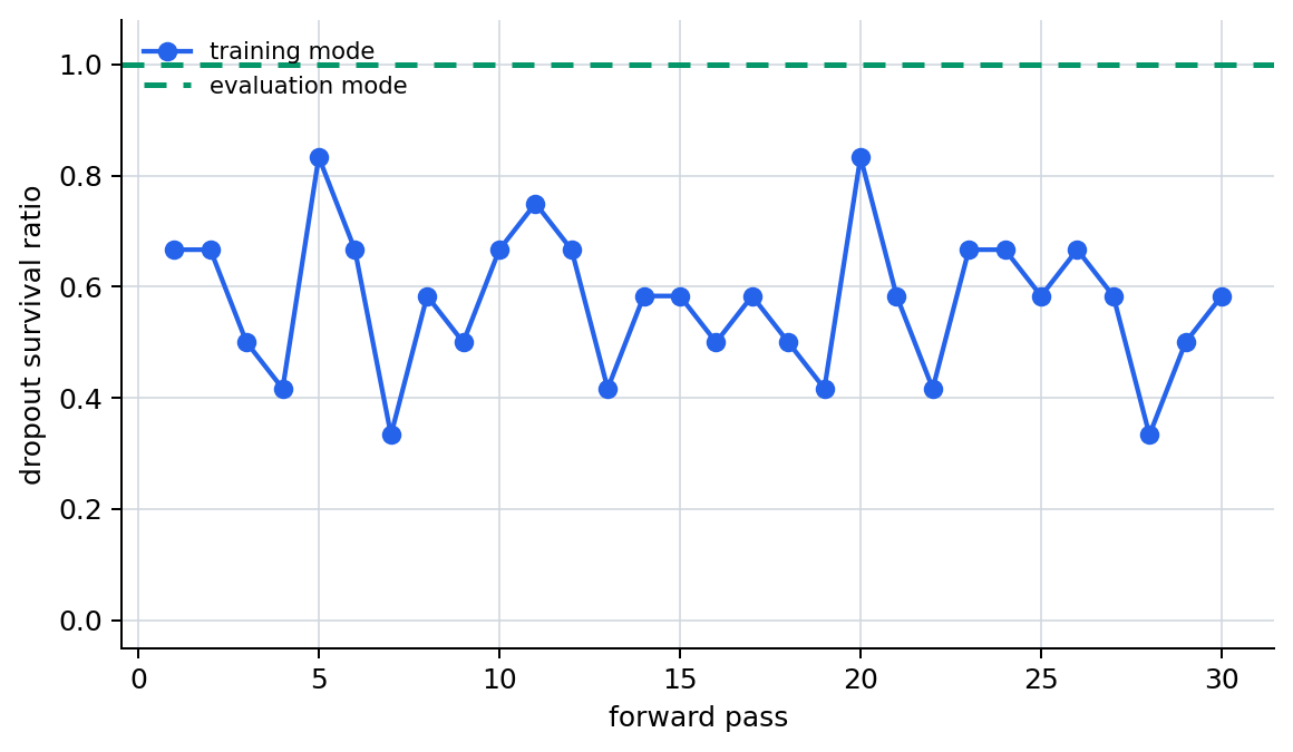
If the two graphs above are the direct explanation of the example code, then the two graphs below are summaries showing how the same phenomenon appears across repeated execution. If we simply draw the two sample-wise lines train_run_1 and train_run_2, it can look like a forced comparison of two hand-picked masks, so instead we apply the same computational rule to a slightly longer mini-batch and summarize only the survival ratio after dropout across 30 forward passes. In training mode, the survival ratio fluctuates by pass, and in evaluation mode dropout is turned off, so the survival ratio stays fixed on the 1.0 baseline.

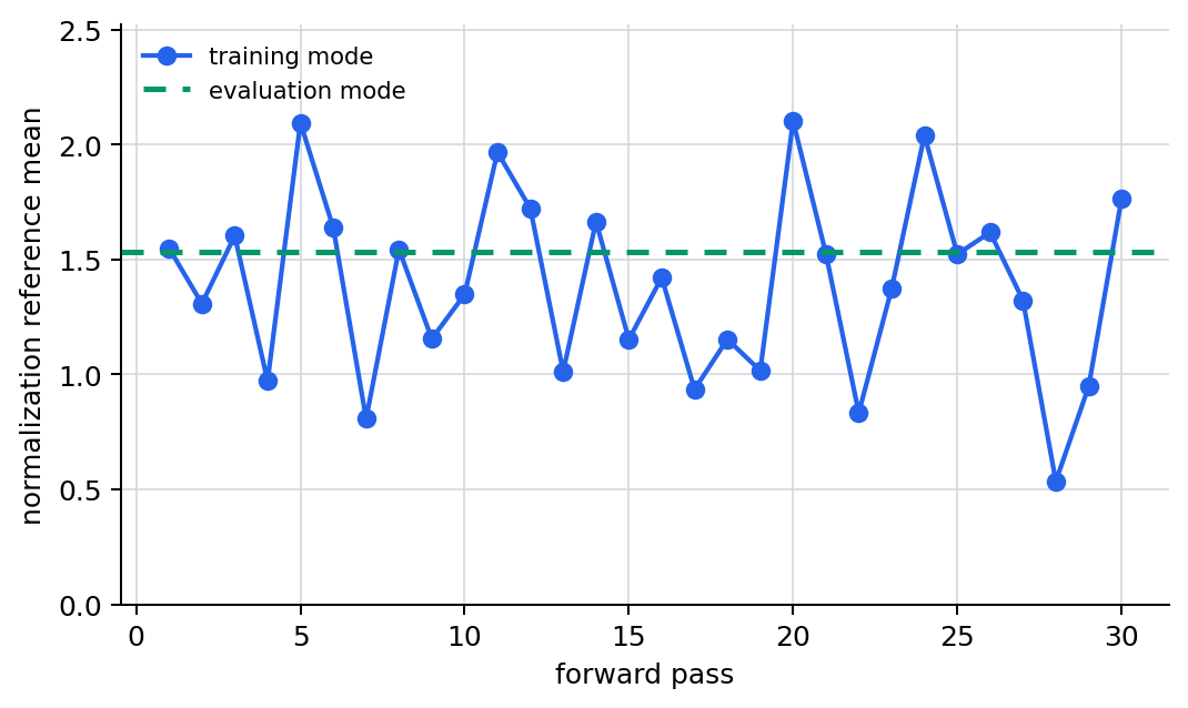
We read the normalization reference the same way. In training mode, the current batch mean computed from the post-dropout values becomes the reference, so the reference mean fluctuates by pass. In evaluation mode, the reference line is not a random mask from the current pass, but the running mean accumulated during learning.

Here too, merely seeing that the output is different is different from reading what computational rule changed because of the mode.

The next thing to confirm from this example is not merely there is a difference, but what gets disturbed by the wrong mode interpretation.

In other words, the experiment in this section does not end at confirming the definition training/eval mode are different. We also have to confirm what breaks interpretation if evaluation is left to fluctuate like training mode. Only then does the need for mode separation become clear.

As deep learning became deeper and model scale grew larger, it became harder to explain actual learning systems only with the sentence the weights are learned. As regularization, normalization, and batch-based training became widely used, the need grew to state clearly in the curriculum that behavior differs between training and evaluation.

In particular, dropout became widely known as a practical technique for reducing overfitting, and batch normalization also appeared often in discussions of deep-network stability and speed. Because of that flow, it became natural in modern deep-learning education to introduce training/eval mode as a separate concept.

In other words, this section is not just a library tip. It is the section that explains why deep learning can look less like a simple function and more like a system with operational states.

When Do We Read The Training/Eval Mode Difference Separately¶

After distinguishing learning and inference, we next have to check separately even for the same model, can some computational rules differ? That boundary is exactly training/eval mode.

Checklist¶

• Can you explain why training mode and evaluation mode can have different computational rules?
• Can you say why the mode distinction matters in dropout or batch normalization?
• Can you explain that training mode and evaluation mode are two different computational states of the same model?
• Can you say that dropout and batch normalization are representative examples that are especially sensitive to the mode difference?
• Can you explain that in validation, test, and deployment, evaluation mode matters because we need to check whether the same input yields a more stable output with less fluctuation?
• When the result feels different between training and validation for the same input, can you first recall the difference between training mode and evaluation mode?
• When you need to reduce output fluctuation in validation and deployment, can you bring out the viewpoint that evaluation mode provides a stable reference?
• Do you understand that after this section, the flow moves on to the optimizer chapters that turn gradients into actual update rules?

Sources And Further Reading¶

• Ian Goodfellow, Yoshua Bengio, Aaron Courville, Deep Learning, MIT Press, 2016, accessed 2026-06-29. https://www.deeplearningbook.org/
• Nitish Srivastava et al., Dropout: A Simple Way to Prevent Neural Networks from Overfitting, JMLR, 2014, accessed 2026-07-19. https://jmlr.org/papers/v15/srivastava14a.html
• Sergey Ioffe, Christian Szegedy, Batch Normalization: Accelerating Deep Network Training by Reducing Internal Covariate Shift, ICML, 2015, accessed 2026-07-19. https://arxiv.org/abs/1502.03167