P5-7.3 Intuition For Adaptive Updates: Adam As An Example¶

Section ID: P5-7.3 Version: v2026.07.20

In P5-7.2, we saw how the actual update step size can differ depending on the learning rate even with the same gradient. From here, the next question appears immediately. Is it enough to apply that step size to every parameter in exactly the same way all the time?

Adaptive update appears exactly at this point. If the basic direct update is a way of moving once based on the current gradient and learning rate, then adaptive update tries to adjust the actual movement amount while also looking at recent gradient flow and parameter-by-parameter differences.

In this section, we use Adam (Adaptive Moment Estimation) as a representative example to read that intuition. The center is not the name Adam itself, but why do recent flow and coordinate-wise adjustment enter the update rule?

If the difference between basic updates and adaptive updates starts to blur together again, return together to the gradient descent and optimizer entries in the concept glossary.

The Question Of What Adam Adapts¶

What does adaptive update try to additionally compensate beyond a basic gradient update?
What is the core intuition of adaptive update in terms of recent gradient flow and coordinate-wise adjustment?
In explaining that adaptive-update intuition, how does Adam become a representative example?
Even though Adam is often mentioned in practice, why should we not memorize it as an absolute winner?

This section explains the problem awareness from which adaptive update comes, rather than increasing the list of optimizer names. What we need to read here is by what rule is the already-computed gradient turned into the actual update, and why recent flow and coordinate-wise differences enter that rule. Adam is used as a representative example for holding onto this intuition. A comparison that first distinguishes optimizer family names continues in the supplementary study of P5-7.5, and optimizer state and parameter-wise update reconnect again in the supplementary study of P5-7.7. The viewpoints of regularization and generalization reconnect in P5-8.1 and P5-8.2, and the convergence analysis of adaptive optimization continues in the supplementary study of P5-7.4.

What to distinguish in this section now	Why it matters
model structure	because it is the question of how to represent the input structure, such as CNN, RNN, or Transformer
optimizer procedure	because it is the question of by what stride length and accumulation rule the parameters are actually moved even for the same structure
difference from regularization	because the optimizer deals with `how should we move`, while regularization deals with `what kinds of solutions should we prefer less`

Standards For Gradient History And Step-Size Adjustment¶

You can explain adaptive update as an update method that reflects recent gradient flow and coordinate-wise adjustment.
You can understand the difference between a basic direct update and an adaptive update.
You can say why Adam is often mentioned as a representative example of adaptive update.
You can confirm the difference in update intuition with an executable Python example.

The Baseline Needed First To Understand Adaptive Update¶

If we start adaptive update immediately from formulas, beginners can easily miss what exactly was added. So we first place the simplest possible baseline. What we have to hold first here is not a specific optimizer name, but the basic feeling that we move once directly based on the current gradient and the learning rate.

It is enough to understand it like this.

Move one step in the direction pointed to by the current gradient, with the amount set by the chosen learning rate.

This intuition continues directly from the explanation in P5-7.2 that the learning rate decides the update stride length. If P5-7.2 explained the stride itself, here we take as the baseline a basic update that applies that stride directly to all parameters in the same way.

The reason we do not place a specific optimizer name first here is also clear. What we need now is not name classification, but the thinnest possible baseline for reading what adaptive update additionally tries to compensate.

the intuition is clear
the core idea of gradient descent becomes visible
and the update rule can be seen most directly

In other words, the baseline of this section is not an introduction to a specific optimizer, but the simplest direct-update intuition used to explain adaptive update.

What Does Adaptive Update Try To Compensate Further¶

Adaptive update uses more information than a simple current-gradient-based update. If we take Adam as the representative example, it is enough to understand the following.

it looks at recent gradient directions in accumulated form
it tries to adjust the amount of change differently by coordinate
and it has the practical purpose of making early learning faster and more stable

In other words, adaptive update tries to reflect information that can easily be missed by only moving every parameter with the same reference stride.

If we reduce it to one sentence, it becomes the following.

Adam is an optimizer that tries to move each parameter more adaptively by referring together to the recent flow of the gradient and to coordinate-wise magnitude differences.

If we make it a little more intuitive, it becomes:

basic update baseline: take a step with the same reference stride in the direction of the slope visible right now
Adam: also look at the wobble of the last few steps, and adjust the stride differently by coordinate

For example, suppose one parameter keeps fluctuating with a large gradient, while another parameter moves very slightly and stably. A basic direct update pushes both using the same learning-rate reference. An adaptive update like Adam, on the other hand, tries to also reflect is this coordinate fluctuating too strongly right now? and is this coordinate moving too slowly? So adaptive update feels closer to a different stride for each coordinate than to the same single step everywhere.

What Do We See About Adaptive Update When We Use Adam As The Example¶

At the introductory stage, the following table matters more than a complicated formula.

Item	Basic direct-update baseline	Adam
basic feeling	one simple one-step update	an adaptive update reflecting more accumulated information
advantage	the intuition is simple and the reference point is clear	the early part of learning is often fast and practically convenient
caution	can be sensitive to learning-rate setting	even if it looks convenient, we still cannot conclude that final generalization is always better

The key in this table is not which one is absolutely superior. Rather, it is safer to understand it like this.

Adam is a representative example that adds recent flow and coordinate-wise adjustment to a simple gradient-update baseline in order to make a more adaptive update.

Why Is Adam So Often Mentioned As The Representative Example¶

Adam is often mentioned in practice. What the reader should hold onto for a long time here is not it is used a lot, but why is it often chosen as the representative example of adaptive update.

it often works reasonably well even from initial settings
it can easily give the experience that the loss decreases quickly in the early part of training
and with large models or complex data it can feel like the barrier to entry is lower

But there is an important caution here.

Just because Adam is often used, that does not guarantee that it always gives a better final result on every problem.

In other words, Adam's popularity comes in large part from practicality and convenience, and different problems still require different judgment.

If we compress everything up to this point once, adaptive update is a method that adds recent flow and coordinate-wise adjustment on top of a basic direct update, and Adam is a representative example that makes that intuition easy to read.

If we compress this difference down to only the update rules, it becomes the following.

flowchart TD
  subgraph SGD["Direct update intuition"]
    direction TB
    A["Current gradient"] --> B["One learning rate"]
    B --> C["Direct update step"]
  end

  GAP["Comparison focus: how the same gradient becomes a step"]

  subgraph Adam["Adam intuition"]
    direction TB
    D["Current gradient"] --> E["Recent gradient history"]
    E --> F["Coordinate-wise adjusted step"]
  end

  SGD --> GAP --> Adam

The first result to confirm in this diagram is that the basic direct update is closer to the feeling of reacting to the current gradient with the same reference stride, while Adam is closer to the feeling of adjusting the stride by reflecting recent flow and coordinate-wise differences more strongly.

Practice And Example¶

We can move directly to the example now. The example in this section is not a full implementation of real Adam; it is a simplified example that isolates the core intuition of adaptive update. The example data is in optimizer-gradient-history.csv. This file contains the gradient flow received by three parameters over 12 steps. One coordinate has a large gradient that steadily shrinks, one has a small gradient that steadily shrinks, and one has a gradient whose direction keeps wobbling.

Input:

gradient flow by parameter recorded across multiple steps
parameter name parameter_name
learning step step
each step's gradient

Output:

parameter movement results from a simple direct-update method
update results from a simplified Adam-like accumulated average and second moment
mean direct_delta and adam_like_delta by parameter
how movement paths differ for large gradients, small gradients, and wobbling gradients

Problem scene:

the difference in adaptive update is easier to read from how parameter-wise gradient flow turns into step-by-step updates than from formula names

Concepts to confirm:

a simple direct update reacts immediately to the current gradient
an Adam-like method adjusts the movement amount by accumulating recent gradient information
an Adam-like method also tries to reflect coordinate-wise gradient magnitude differences in the size of the update

Input:

The CSV contains gradient flows for the following three coordinates.

Parameter	Gradient flow	What to predict first
`risk_weight`	large negative gradients steadily shrink	the direct update moves far, while the Adam-like update adjusts the stride by looking at magnitude history
`recovery_weight`	small negative gradients steadily shrink	the direct update barely moves, while the Adam-like update adjusts even the small coordinate by its own history
`noise_weight`	negative and positive gradients alternate	the direct update keeps changing direction, while the Adam-like update accumulates recent flow and reduces wobble

The purpose of this table is not to memorize exact numbers in advance. It is to hold before the code that even with the same learning rate, a simple direct update reflects the current gradient immediately, while Adam-like keeps recent flow and coordinate-wise magnitude history and can create a different movement path.

# This example reads CSV gradient history and compares how direct updates and
# Adam-like updates create different parameter movement paths.
from csv import DictReader
from pathlib import Path

DATA_PATH = Path("docs/assets/part-05/chapter-07/optimizer-gradient-history.csv")
PARAMETER_ORDER = ["risk_weight", "recovery_weight", "noise_weight"]


def load_rows(path):
    with path.open(newline="", encoding="utf-8") as f:
        return [
            {
                "step": int(row["step"]),
                "parameter_name": row["parameter_name"],
                "signal_group": row["signal_group"],
                "gradient": float(row["gradient"]),
            }
            for row in DictReader(f)
        ]


def simulate_updates(rows):
    learning_rate = 0.05
    beta1 = 0.8
    beta2 = 0.9
    epsilon = 1e-8
    state = {
        parameter_name: {
            "direct_weight": 1.0,
            "adam_like_weight": 1.0,
            "m": 0.0,
            "v": 0.0,
        }
        for parameter_name in PARAMETER_ORDER
    }
    simulated = []

    parameter_index = {
        parameter_name: index
        for index, parameter_name in enumerate(PARAMETER_ORDER)
    }
    for row in sorted(
        rows,
        key=lambda item: (item["step"], parameter_index[item["parameter_name"]]),
    ):
        parameter_name = row["parameter_name"]
        gradient = row["gradient"]
        parameter_state = state[parameter_name]

        direct_delta = -learning_rate * gradient
        parameter_state["direct_weight"] += direct_delta

        parameter_state["m"] = beta1 * parameter_state["m"] + (1 - beta1) * gradient
        parameter_state["v"] = (
            beta2 * parameter_state["v"]
            + (1 - beta2) * gradient * gradient
        )
        adam_like_delta = (
            -learning_rate
            * parameter_state["m"]
            / (parameter_state["v"] ** 0.5 + epsilon)
        )
        parameter_state["adam_like_weight"] += adam_like_delta

        simulated.append(
            {
                "step": row["step"],
                "parameter_name": parameter_name,
                "gradient": gradient,
                "direct_delta": direct_delta,
                "adam_like_delta": adam_like_delta,
                "direct_weight": parameter_state["direct_weight"],
                "adam_like_weight": parameter_state["adam_like_weight"],
            }
        )

    return simulated


rows = load_rows(DATA_PATH)
simulated = simulate_updates(rows)

print("[input]")
print("rows =", len(rows))
print("parameters =", ", ".join(PARAMETER_ORDER))

print("\n[checkpoints]")
for item in simulated:
    if item["step"] in [1, 6, 12]:
        print(
            item["parameter_name"],
            "step =", item["step"],
            "gradient =", item["gradient"],
            "direct_delta =", round(item["direct_delta"], 3),
            "adam_like_delta =", round(item["adam_like_delta"], 3),
        )

print("\n[final weights]")
for parameter_name in PARAMETER_ORDER:
    last = [
        item for item in simulated
        if item["parameter_name"] == parameter_name
    ][-1]
    print(
        parameter_name,
        "direct_weight =", round(last["direct_weight"], 3),
        "adam_like_weight =", round(last["adam_like_weight"], 3),
    )

In the output, first compare how the step-by-step updates of the simple direct update and the Adam-like method differ even under the same CSV input.

[input]
rows = 36
parameters = risk_weight, recovery_weight, noise_weight

[checkpoints]
risk_weight step = 1 gradient = -7.0 direct_delta = 0.35 adam_like_delta = 0.032
recovery_weight step = 1 gradient = -0.6 direct_delta = 0.03 adam_like_delta = 0.032
noise_weight step = 1 gradient = -3.0 direct_delta = 0.15 adam_like_delta = 0.032
risk_weight step = 6 gradient = -3.0 direct_delta = 0.15 adam_like_delta = 0.049
recovery_weight step = 6 gradient = -0.29 direct_delta = 0.014 adam_like_delta = 0.05
noise_weight step = 6 gradient = 1.2 direct_delta = -0.06 adam_like_delta = -0.001
risk_weight step = 12 gradient = -0.4 direct_delta = 0.02 adam_like_delta = 0.03
recovery_weight step = 12 gradient = -0.05 direct_delta = 0.003 adam_like_delta = 0.034
noise_weight step = 12 gradient = 0.3 direct_delta = -0.015 adam_like_delta = -0.0

[final weights]
risk_weight direct_weight = 2.87 adam_like_weight = 1.502
recovery_weight direct_weight = 1.171 adam_like_weight = 1.52
noise_weight direct_weight = 1.07 adam_like_weight = 1.063

If we separate even the same output into input gradient -> step-by-step update -> accumulated weight, it becomes clearer what the Adam-like method is trying to compensate further.

Parameter-wise gradient flow

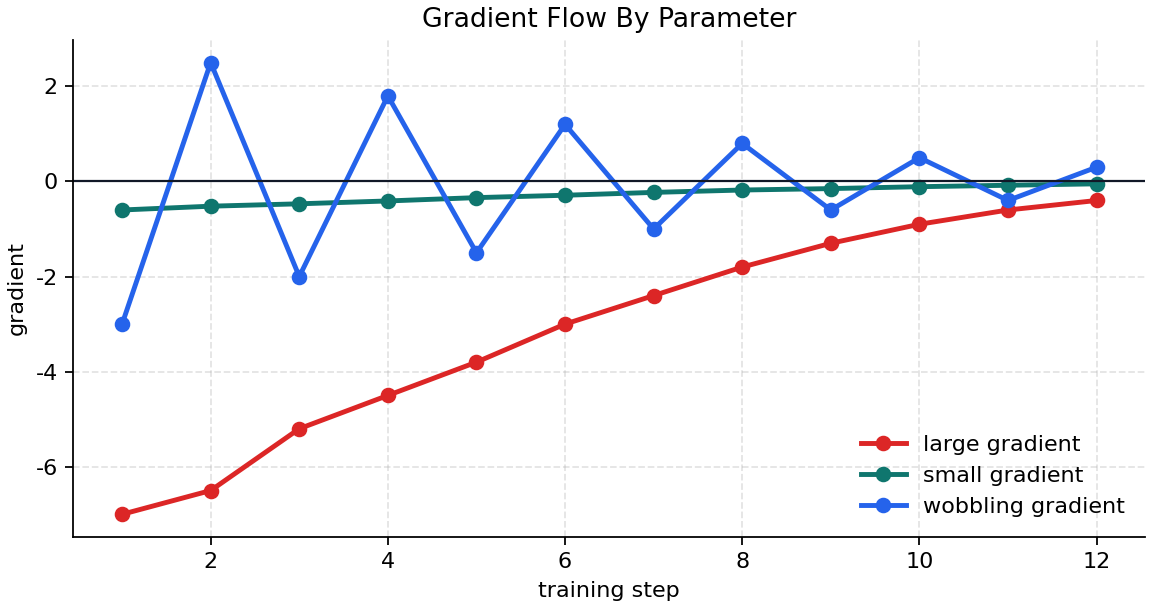
The input at the first stage is the gradient flow before the optimizer changes anything. risk_weight has a large negative gradient that steadily shrinks, recovery_weight has a small negative gradient that steadily shrinks, and noise_weight keeps changing direction. The simple direct update and the Adam-like method both receive this same input.

Mean update scale by coordinate

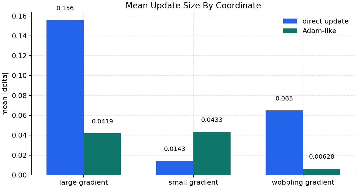
The difference appears at the delta stage. The simple direct update transfers gradient magnitude differences almost directly into update magnitude differences. Because the Adam-like method uses recent flow and coordinate-wise magnitude history together, the coordinate with a large gradient is relatively suppressed, and the coordinate with a small gradient is also adjusted against its own history.

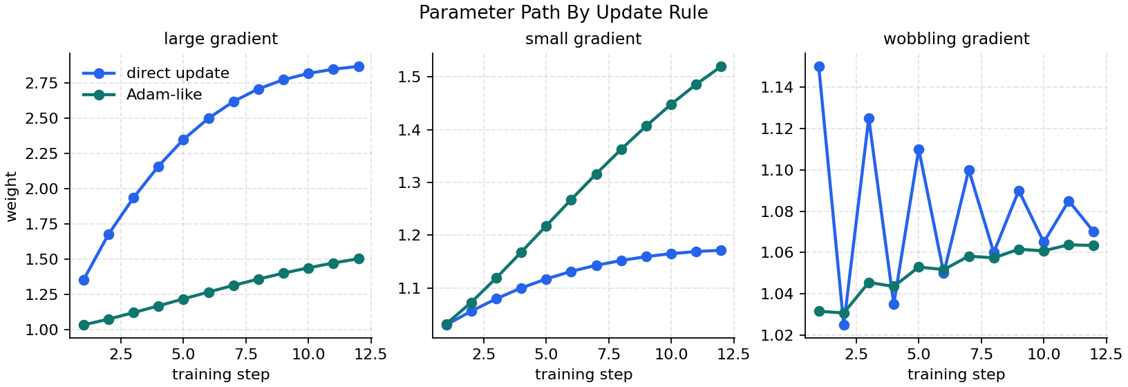
Parameter movement path by update rule

If we look at the final parameter paths, this difference accumulates. For risk_weight, where the large gradient is steady, the direct update moves much farther. For recovery_weight, where the small gradient is steady, Adam-like reacts more strongly. For noise_weight, whose direction wobbles, neither path moves very far. What changes at this stage is not that the gradient was newly computed, but the way the optimizer rule turns the same gradient flow into an actual parameter path.

This example is neither a full implementation of real Adam nor an experiment that judges the performance superiority of a simple direct update versus Adam. The core point to read here is the following.

the simple direct update reflects the current gradient relatively directly
the idea of Adam-like methods is to accumulate recent directions and coordinate-wise magnitude histories, thereby making step-by-step updates different
an optimizer does not merely decrease something, but decides through what update path should the same gradient be turned

After reading this example, the compensations of adaptive update divide into two axes.

Axis to read	Change to check directly	Sentence to leave from this section
time axis	recent gradients remain in the moving average, so the step-by-step update becomes smoother	adaptive update can look at recent flow rather than only at the current gradient
coordinate axis	each parameter separately accumulates its own gradient magnitude history and adjusts the stride	adaptive update does not push all parameters only with the same reference stride

Once this table is read, the core of adaptive update should be explainable as a method that puts both time-axis accumulation and coordinate-axis adjustment into the update rule. It is enough to summarize Adam as a representative example that shows that method.

When Do We First Bring Out The Adaptive-Update Viewpoint¶

After understanding the general role of the optimizer, it is helpful to read separately is the basic update intuition enough here, or is the adaptive-update intuition needed?

Problem scene that appears first	Optimizer viewpoint to recall first	Reason
we need to explain the most basic structure of gradient direction and step size	simple update baseline	it shows most clearly the basic update intuition that reacts directly to the current gradient
early learning is too rough, or coordinate-wise scale differences are large	adaptive update	the intuition of updates that reflect accumulated information and coordinate-wise adaptation becomes more important
we need to explain why Adam is often used in practice	recall adaptive update first, and see Adam as a representative example	convenience and practicality are important, but if the representative example is immediately confused with the general principle, the intuition blurs
there is a tendency to memorize optimizers as an absolute ranking	place the simple baseline and adaptive update side by side	because speed, stability, and generalization have to be read separately

Checklist¶

Can you explain what adaptive update is trying to additionally compensate beyond the basic update?
Can you explain that adaptive update is a method that reflects accumulated information and coordinate-wise adjustment more strongly?
Can you explain the difference between a simple update baseline and an adaptive update as the difference between reacting directly to the current gradient and reflecting accumulated information and coordinate-wise differences more strongly?
Can you distinguish that the first example should be read as time-axis accumulation, and the second example as coordinate-axis adjustment?
Can you say that Adam is only a representative example of adaptive update, and cannot be concluded to be an absolutely better optimizer?

Sources And Further Reading¶

Léon Bottou, Large-Scale Machine Learning with Stochastic Gradient Descent, COMPSTAT, 2010, accessed 2026-07-19. https://doi.org/10.1007/978-3-7908-2604-3_16
Diederik P. Kingma, Jimmy Ba, Adam: A Method for Stochastic Optimization, arXiv, 2014, accessed 2026-07-19. https://arxiv.org/abs/1412.6980
Sebastian Ruder, An overview of gradient descent optimization algorithms, arXiv, 2016, accessed 2026-07-19. https://arxiv.org/abs/1609.04747