P5-7.6 Supplementary Reading: Learning-Rate Control Strategies
Section ID:
P5-7.6Version:v2026.07.26
In P5-7.2, we read the learning rate as the stride length of one update. But once we look at actual training settings, we meet scenes where the learning rate is not fixed from beginning to end and instead keeps changing under names such as warmup, decay, and cosine schedule.
The question the reader should hold onto immediately here is not did another new optimizer appear?, but even while using the same optimizer, why is the stride-management policy made different over time? This viewpoint also becomes a reusable standard later when reading training logs, fine-tuning settings, and experiment tables in papers, because it lets us separate optimizer choice from stride-management policy.
The Question That Needs a Learning-Rate Schedule
- Why do we distinguish a fixed learning rate from a learning rate that changes over time?
- Why should warmup be read as a device that gradually increases the stride at the beginning?
- Why should decay be read as a device that decreases the stride later?
- Can we distinguish scheduler families not through formula memorization, but through
stride-management patterns?
This section focuses not on the implementation API of schedulers, but on explaining how we should manage the stride during the early phase of learning, the middle phase of learning, and the later phase of learning.
Standards for Warmup and Decay
- You can explain a learning rate scheduler as
a stride-management policy. - You can say what kind of training-stage problem warmup and decay each try to alleviate.
- You can distinguish step decay, linear decay, and cosine decay at a broad level.
- You can explain when scheduler questions should be brought out first while reading a training log.
Why Doesn't the Explanation End With a Fixed Learning Rate
A fixed learning rate is very appropriate for the introductory explanation in P5-7.2. But in actual learning, it is not always the case that the same stride is good across every interval.
- in the early phase, parameters can still fluctuate roughly
- in the middle phase, a stride that advances quickly can be advantageous
- in the later phase, a stride that finely adjusts small differences can be better
So it is safer to read a scheduler not as a device that changes the optimizer, but as the device that decides what stride policy the same optimizer will use on the time axis of learning.
If we unpack this sentence more directly, it becomes the following. The optimizer decides how should we move, while the scheduler decides when should we move largely, and when should we move finely. The two are not on the same layer. We can change the scheduler without changing the optimizer, and we can change only the optimizer while keeping the same scheduler. This distinction has to be fixed first so that phrases such as use Adam, use cosine decay, and add warmup do not blur into the same kind of choice.
Another important point is that, when understanding a scheduler, we do not need a complicated formula from the start. What we have to look at first is on the time axis of learning, do we decide one stride once and end there, or do we operate it differently by interval? Once that question is clear, then even if a library function name appears later, the reader does not get lost.
It becomes simpler if we turn it into one small scene. Suppose we train the same model for 10 minutes. The first 1 minute may be a stage where the model is still finding its direction, the middle 6 minutes may be the stage where it is reducing quickly, and the last 3 minutes may be the stage where it is refining near a fairly good region. If these three intervals feel different from one another, then the question is it really natural to keep exactly the same stride for the whole training run? becomes the exact starting point of the scheduler.
This scene matters because when beginners first learn the learning rate, they easily remain with the feeling we choose one number. But once the scheduler enters, the question changes. Now it is no longer what number should we choose, but should we keep this number unchanged for the whole learning process? Once the reader crosses only this one step, scheduler documents feel far less abrupt.
One Very Small Numeric Example. The Difference Between A Fixed Learning Rate And A Schedule
For example, suppose training lasts for 6 steps, and the base learning-rate candidate is 0.1.
| step | fixed learning rate | warmup + decay example |
|---|---|---|
| 1 | 0.1 | 0.02 |
| 2 | 0.1 | 0.06 |
| 3 | 0.1 | 0.10 |
| 4 | 0.1 | 0.08 |
| 5 | 0.1 | 0.05 |
| 6 | 0.1 | 0.02 |
The core shown by this table is simple. A fixed learning rate reads every step with the same stride. By contrast, warmup + decay reads it as carefully at first, fully in the middle, and carefully again near the end. If a beginner only holds onto this feeling, scheduler names already become much less abstract.
The difference becomes more direct if we look at it through a graph.
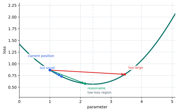
Even on the same loss curve, if the stride is too small, it barely moves; if it is appropriate, it goes toward lower loss; if it is too large, it can overshoot. A scheduler is the device that widens this stride question into how should we operate the stride over the whole time axis of learning?
Why Is Warmup Needed
Warmup is the method of not setting the learning rate large from the very beginning, but instead starting from a small value and gradually increasing it over several steps or epochs.
The reason this device is needed is simple. In the early phase of learning, the parameters can still be unstable and the gradient pattern can still be rough. If a large stride is given from the start, the model can swing too aggressively before it has even learned a good direction.
If we reduce it to one sentence, it becomes the following.
Warmup is the device that gradually increases the stride in order to ease the rough movement of the early learning stage.
If we say this more ordinarily, warmup is closer to do not start at full speed right away. At the beginning of learning, the parameters are still coarse in where they are, and the pattern of the gradient is not yet stable either. If a large learning rate is given immediately there, the model can wobble with too large a stride at the stage when it is only beginning to discover the direction. It is enough to see warmup as the device that reduces this early overspeed and gives learning time to settle into a rhythm.
For example, suppose we open a training log and see that in the first several tens of steps the loss fluctuates sharply up and down, and only later becomes somewhat stable. At this point, the reader may first think is the model structure bad? or is the optimizer wrong? But from the warmup viewpoint, the question becomes much simpler. Is the stride too large for something that is still at the beginning? That question is the easiest starting point for recalling warmup.
Said very briefly again, warmup is close to do not take huge steps when we still do not sufficiently know the good direction. Once this one sentence comes in, warmup is read not as a strange device, but like an anti-overspeed device for the beginning.
Why Is Decay Needed
Decay is the policy of reducing the learning rate as learning proceeds. At the introductory stage, it is enough to keep only the following feeling.
- in the early phase, moving more largely can be acceptable
- in the later phase, since we may already be near a good region, smaller strides can be better for fine adjustment
In other words, it is enough to read decay as reducing the stride when moving into later fine-tuning mode.
If we unpack this one more time, decay reflects the fact that continuing to move largely is not always good. In the early phase of learning, it may matter to reduce coarse errors quickly, but in the later phase, the model may already be near a fairly good position. If we still keep moving with a large stride there, we may overshoot the target area or keep small oscillations for a long time. Decay is best read as the policy now let us move more carefully in exactly this later interval.
This too becomes easier if we turn it into a small scene. In the early phase, a loss going 16 -> 9 -> 4 quickly downward feels welcome. But in the later phase, a scene such as 0.8 -> 0.6 -> 0.7 -> 0.5, rising and falling near the target region, becomes more important. At that stage, go faster matters less than do not overshoot. Decay is the device that corresponds exactly to this later-phase feeling.
Said very briefly again, decay is close to once we are near a good place, shorten the step. If warmup prevents early overspeed, decay stands on the side of reducing later over-oscillation.
How Do We Distinguish Scheduler Patterns Differently
| Name | Feeling to read first | How the stride changes |
|---|---|---|
| step decay | reduce it like stairs | lower it once by a large amount at fixed points |
| linear decay | reduce it gradually like a straight line | decrease it steadily over time |
| cosine decay | reduce it more softly toward the end | decrease it like a smooth curve |
| warmup + decay | raise it early, then reduce it later | an increasing interval followed by a decreasing interval |
This table does not say which formula is more elegant. It is a table that helps the reader, when seeing the name, first recall when does the stride increase, and when does it decrease?
For a beginner, it is better not to read this table as a formula table. It is closer to an operations table that writes down how will we change the stride on the time axis of learning?
Reading It Again as Stride-Management Patterns
| Learning interval | Stride-management question | Device often connected |
|---|---|---|
| early phase | if we move largely from the start, will it be too rough? | warmup |
| middle phase | do we need an interval that advances quickly? | maintain a relatively large base learning rate |
| later phase | do we need to move more finely to avoid overshooting near the target? | decay |
Seen this way, a scheduler is not a new optimizer, but the rule for operating stride over time on top of one optimizer.
If we miss this distinction, the reader can easily accept we decided the learning rate and we decided the learning-rate schedule as if they were the same statement. But in reality they are different. The former decides the basic size of the stride now, while the latter decides how that stride will be changed over the whole learning run. These two have to look separate so that later, when reading a paper or practical setting, a sentence such as optimizer is Adam, scheduler is cosine, warmup is 5% can be decomposed naturally.
Cases and Examples
Case. The Same Optimizer, But Different Problems Appear In The Early And Later Phases
Even if we choose one optimizer such as Adam or momentum, the problems seen in the early phase and the later phase can be different. For example, in the early phase the loss can jump strongly, in the middle phase it can go down quickly, and in the later phase small oscillations can remain for a long time near the target.
If we read every one of these scenes only as is the optimizer bad?, the interpretation becomes too large and lumped together. The scheduler viewpoint breaks the question into smaller ones.
| Scene we see | Scheduler question to recall first | Reading standard |
|---|---|---|
| the early loss fluctuates strongly | is the initial stride too large? | is warmup needed? |
| the middle phase goes down well, but later oscillation is large | is the later stride still too large? | is decay needed? |
| the whole learning run is too slow | is the stride too small from beginning to end? | is the base learning rate or the whole schedule too conservative? |
What the current section has to close is not which scheduler is famous, but do we read stride-management questions separately on the time axis?
If we unpack this case more, what is hard for a beginner when reading an actual log is not the number itself, but the timing. Even on the same loss curve, the strong fluctuation in the early phase and the small oscillation in the later phase may not have the same cause. That is why the scheduler viewpoint first makes us ask in what interval is the problem appearing right now? If it is the aggressiveness of the beginning, then the warmup question appears first. If it is the remaining small oscillation in the later phase, then the decay question appears first. Once the time axis is split first, guessing the cause becomes far less lumped together.
Practice and Example
Read the following log-interpretation sentences and write down what stride-management pattern should be checked first.
| Log-interpretation sentence | Scheduler question to check first | Device to recall first |
|---|---|---|
| In the first several hundred steps, the loss curve is very rough | should the stride be increased more gradually in the early phase? | warmup |
| Even after it has already become good enough, the up-and-down oscillation near the target remains large | should the later stride be reduced more? | decay |
| After a certain milestone, we want to move into finer adjustment | should we lower the stride step by step by interval? | step decay |
| We want to reduce it smoothly over the whole training run | should we reduce it continuously rather than in stairs? | linear/cosine decay |
The purpose of this exercise is not to memorize scheduler names, but to build the habit of first recalling the stride-management question.
Checklist
- Can you explain a learning rate scheduler as
a stride-management policy? - Can you explain warmup as
a device that stops the model from moving too largely all at once in the early phase? - Can you explain decay as
a stride reduction for later fine adjustment? - Can you read step decay, linear decay, and cosine decay as
stride patterns? - When reading a training log, can you connect early instability, later oscillation, and overall overspeed/underspeed to scheduler questions?
Sources and References
- PyTorch,
torch.optim, PyTorch documentation. Referenced to confirm thatlr_scheduleradjusts the learning rate according to epochs or validation metrics, and that PyTorch provides schedulers such asStepLR,LinearLR, andCosineAnnealingLR. Checked: 2026-07-19. https://docs.pytorch.org/docs/stable/optim.html#how-to-adjust-learning-rate - Ilya Loshchilov, Frank Hutter,
SGDR: Stochastic Gradient Descent with Warm Restarts, ICLR 2017. Referenced to confirm background on cosine annealing and restart-style learning rate schedules. Checked: 2026-07-19. https://arxiv.org/abs/1608.03983