P5-7.7 Supplementary Reading: Optimizer State and Per-Parameter Updates
Section ID:
P5-7.7Version:v2026.07.26
In P5-7.3, when we looked at adaptive updates, the expressions recent gradient flow and coordinate-wise adjustment kept appearing. The natural question left from there is this. Where is that kind of information left, and why can the next update differ even when the same gradient comes in?
To answer this question, we have to distinguish parameter, gradient, update, and optimizer state from one another. This distinction keeps being reused later too when we look at checkpoint saving, training restart, optimizer replacement, and fine-tuning settings.
The reason this section feels compressed to beginners is that all four words look like similar numbers. Even in actual code, these values appear together in similar lines, so at first they easily feel like the same thing being called by different names.
The Question of How Optimizer State Changes Updates
- What are parameter, gradient, update, and optimizer state respectively?
- Why is optimizer state different from model parameters?
- When we say parameter-wise update, what does it mean that something is kept separately by coordinate?
- Why does an adaptive optimizer look together not only at
the current gradient alone, but also atits accumulated internal state?
This section focuses not on library implementation details, but on explaining what the optimizer is keeping separately in memory.
Standards for Parameter-Wise State and Application Units
- You can distinguish parameter, gradient, update, and optimizer state.
- You can explain that optimizer state can be maintained separately by coordinate.
- You can say that even with the same gradient, the next update can differ when the state differs.
- You can explain that the
adaptivein an adaptive optimizer is connected to the accumulation of internal state.
We First Have to Separate Four Things
| Item | What it is | When it changes |
|---|---|---|
| parameter | the weight value the model actually holds | when the optimizer reflects the update |
| gradient | the direction signal computed at the current parameter | when backward is performed |
| update | the movement amount to be applied to the parameter in this step | when the optimizer reads the gradient and the state |
| optimizer state | the internal memory the optimizer keeps for the next step | it can be updated together after each step |
If we bundle this table into one sentence, it becomes the following.
The gradient is the signal, the update is the movement amount, the parameter is the actual value, and the optimizer state is the memory left behind for making the next movement.
This one sentence matters because, when beginners look at learning code or explanatory sentences, they easily feel these four as almost the same kind of object. In particular, if phrases such as the gradient was computed, the optimizer ran, and the model was updated appear in sequence, they can look like very similar statements. But in reality, they are different layers. The gradient is the signal at the current position, the update is the movement amount that will actually be applied in this step after receiving that signal, the parameter is the result after that movement amount is reflected, and the optimizer state is the internal memory kept separately for the next step.
This distinction has to settle in the reader's mind so that confusion is reduced even when reading adaptive optimizers later. Only then do sentences such as Adam carries more state, it makes a parameter-wise update, and even with the same gradient the update differs continue naturally into one another.
How Should We Split Three Lines Of Learning Code When We Read Them
Beginners easily read the three sentences below as if they were almost the same event.
| Phrase seen in code or explanation | What actually happened |
|---|---|
| computed the gradient | computed the signal for which direction is good at the current position |
| the optimizer took a step | used that signal and the state to make and reflect this step's movement amount |
| the model was updated | the parameter values themselves changed |
Once this table is placed first, it becomes much clearer that the optimizer and the update sit in between the gradient was computed and the parameter changed.
If we compress it into a diagram, then even inside the same learning loop the four items occupy different places as follows.
flowchart TD
  A["forward pass<br/>predict with current parameters"]
  B["loss<br/>measure error as a number"]
  C["backpropagation<br/>compute gradients"]
  D["optimizer<br/>turn gradients into an update"]
  E["parameter update applied<br/>weights actually change"]

  A --> B
  B --> C
  C --> D
  D --> E

  B -. "what is wrong" .-> C
  C -. "which direction should change" .-> D
  D -. "apply the computed result as an actual move" .-> E
The especially important interval for the current section in this diagram is gradient computation -> optimizer -> parameter application. It is enough to read optimizer state here as the internal memory that helps answer into what movement amount should we turn this signal now?
Why Does Optimizer State Have to Be Separate
For a basic direct update, the current gradient and the learning rate can be enough to make an update. But if we want to reflect recent flow or coordinate-wise magnitude as in momentum, RMSProp, or Adam, then information from previous steps has to be left somewhere. That role is played by the optimizer state.
For example, values such as the following belong to the state.
- the accumulated value of the previous movement direction
- the coordinate-wise average of squared gradients
- auxiliary information needed for step count or bias correction
In other words, optimizer state is not knowledge with which the model represents the world. It is closer to the working memo the optimizer carries in order to decide how should I make the next movement?
If we unpack this analogy more, the model parameters correspond more to how is the current model representing the world, while the optimizer state is closer to the auxiliary record for how should that representation be adjusted next. Because both are numbers, their saved formats can look similar, but their roles are different. Parameters are the content of the model. State is the context of the movement rule.
So the most important attitude when understanding optimizer state is not to mix it together as is this also what the model learned? What the model learned is stored in the parameters, and the information the optimizer temporarily carries to continue the learning process more stably is stored in the state. This separation must be clear so that scenes such as checkpoints, optimizer restart, and fine-tuning become less confusing later.
If we turn it into a small scene, the difference becomes clearer. When saving a model file, what matters is usually what values does the current model hold? But if we want to continue training again from the middle, then not only the model values, but also what flow the optimizer had been remembering so far may be needed. It is exactly there that the distinction parameters are the model content, state is the learning-process context gains real meaning.
One Very Small Numeric Example. When We Look At Parameter And State Together
Suppose there are two coordinates, risk_weight and recovery_weight.
| Item | risk_weight | recovery_weight |
|---|---|---|
| current parameter | 1.4 | 0.8 |
| current gradient | -1.0 | -1.0 |
| example of accumulated state | has received large gradients many times recently | has been almost quiet recently |
On the surface, the current gradients of both look the same as -1.0. But once we read the state row together, the two are no longer standing in the same context. Exactly because of this difference, when we use adaptive optimizers it is safer not to read the current gradient is the same and the next update is the same as the same statement.
What Does Parameter-Wise Update Mean
Parameter-wise update means that not every parameter is moved by one common number only, but that each coordinate can receive a different update according to its own information.
What matters here is that different state can exist for each parameter. One coordinate may have received large gradients many times recently, while another may hardly have moved. Adaptive optimizers keep separate state by coordinate in order to reflect this difference.
So when we see a parameter-wise update, it is safer first to ask the following questions.
- What is stored separately for each coordinate?
- How does that stored value enter into the next update size?
- Even if all coordinates share the same learning rate, why can the actual movement amount still differ?
These questions matter because the intuition all parameters inside the same model always move in the same way does not match actual adaptive optimizers. As the number of parameters grows, some coordinates can see large gradients often, some can receive almost no signal, and some can suddenly react strongly only recently. Parameter-wise update is the expression that recognizes exactly this difference. It does not measure every coordinate with the same ruler. It also looks at the state each coordinate is carrying.
If we read this sentence more practically, parameter-wise update is close to saying not every weight is treated exactly the same. This is not discrimination. It means the update rule recognizes that each coordinate has a different history of response so far. Some coordinates have already moved a lot, some have hardly moved, and some may only recently have started reacting strongly. Adaptive optimizers stand on the side of not ignoring this difference.
If this still feels unfamiliar, we can think of the difference between giving the same homework to the whole class and giving different supplementary work according to what each student is lacking. Parameter-wise update is closer to the latter. It does not treat every coordinate as if it were in the same situation. It reads a different context for each coordinate.
Separating Time-Axis State and Coordinate-Axis State
| Category | What it means | Example |
|---|---|---|
| time-axis state | memory that carries information from previous steps into the current step | accumulated movement direction in momentum |
| coordinate-axis state | memory that is accumulated separately by parameter | the coordinate-wise second moment in Adam |
Actual adaptive optimizers can have both axes together. So the phrase there is state does not merely mean more storage is needed. It also means that the update rule has started reading time and coordinates together.
Why Can the Next Update Differ Even With the Same Gradient
Even when the same gradient comes in again, the update can differ depending on what state was accumulated in previous steps. For example, one coordinate may have a state already formed by repeated large gradients so that it moves more cautiously, while another coordinate may have hardly moved and therefore can still react more strongly.
In other words, in an adaptive optimizer, what is the gradient now alone does not completely determine the next update. The gradient now and the state left over so far together create the next movement amount.
Once this sentence is held, the following distinction becomes clearer.
- the gradient is the input signal of this step
- the optimizer state is the context left from previous steps
- the update is the actual movement amount of this step that comes out after combining the two
If we understand this structure, then the question why does Adam move differently even with the same gradient becomes much easier. The answer is not hidden in a mysterious algorithm name, but in the fact that accumulated context is already attached in front of the current gradient. In other words, an adaptive optimizer does not only react immediately to the current signal. It also reads together the movement history and coordinate-wise response record up to now.
Cases and Examples
Case. Why Does The Update Look Different Even Though The Gradient Is The Same
Suppose two parameters both receive gradient = -1.0 right now. On the surface, it feels as if both should move in the same direction by the same amount, but in an adaptive optimizer that does not have to be true. One parameter may already have received large gradients many times in previous steps, while the other may just now be receiving a large signal for the first time.
If we reread this scene from the viewpoint of state, it becomes the following.
| What is visible now | If we read it without state | If we reread it with state included |
|---|---|---|
| the current gradients of the two coordinates are the same | it feels as if the next updates should also be the same | if the previous accumulated values differ, the updates can differ too |
| one coordinate moves less | it can feel as if the optimizer is ignoring that coordinate | it may simply be being adjusted more conservatively because of already-large accumulated state |
| one coordinate moves more | it can feel unstable | it may be in a state that can still react more strongly because little has been accumulated yet |
What this section has to close is the point that, in an adaptive optimizer, same gradient = same update does not automatically hold.
To make this sentence something the reader can really accept, we need to unpack it one more step. For a beginner's intuition, if the input is the same, the output should also be the same feels natural. But in an adaptive optimizer, the current gradient is not the only input. The state left over from the previous steps is also part of the input. So even if the current gradient is the same, if the state attached before it differs, the update can differ. Once this point becomes visible, sentences about adaptive optimizers feel much less abstract all of a sudden.
If we attach one very small numeric scene, it becomes even easier. Suppose two coordinates both receive the current gradient -1.0. But the first coordinate may have received continuously large signals in the last five steps, such as -3.0, -2.0, and -2.5, while the second coordinate may have stayed near 0.0 for a long time and only this time received -1.0 for the first time. If we look only at the current one-line gradient, the two look the same. But when state is included, the first coordinate may already have a context for moving more cautiously, while the second may still have room to react more strongly. If we imagine this scene, the question why is the update different even though the gradient is the same? feels far less strange.
If we rewrite this example in a table, it becomes the following.
| Coordinate | current gradient | previous context | more natural interpretation |
|---|---|---|---|
| first coordinate | -1.0 | has kept receiving large signals for several recent steps | a state may already be accumulated for moving more cautiously |
| second coordinate | -1.0 | has been quiet for a long time | there may still be room to react more strongly to this signal |
In other words, even if the current input number is the same, to avoid misunderstanding adaptive-optimizer updates we have to read together what kind of context is attached behind this number?
If we look at this difference through a graph again, it becomes more direct.
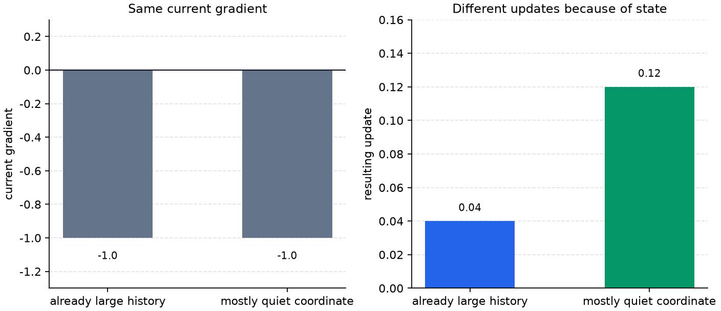
The left panel shows the scene where both coordinates receive the same current gradient -1.0. The right panel shows that even then, the updates can split into 0.04 and 0.12. What changed here is not the current gradient, but the state that had already been attached before it. This graph lets us visually confirm once more that even with the same input, if the context differs, the output can differ.
Practice and Example
Read the following sentences and write down what distinction is missing.
| Sentence | Missing distinction | Standard for reading it again |
|---|---|---|
| Since the gradient was computed, the parameter has now changed | the distinction between gradient and update | was the movement amount made by the optimizer actually reflected? |
| Adam just decides the learning rate automatically | the distinction between state and parameter-wise update | does it adjust the stride by looking at coordinate-wise accumulated state? |
| Since two coordinates received the same gradient, they should receive the same update | the distinction between current gradient and stored state | are the previously accumulated states also the same? |
| Optimizer state is the knowledge the model learned | the distinction between parameter and optimizer state | have we separated the model content from the memory used for the movement rule? |
The purpose of this exercise is not to memorize implementation APIs, but to distinguish what the optimizer stores as actual parameters from what it stores as working memory.
Checklist
- Can you explain parameter, gradient, update, and optimizer state as different things?
- Can you explain that optimizer state is
the internal memory for making the next movement? - Can you say that parameter-wise update connects to the fact that
state can differ by coordinate? - Can you explain that even with the same gradient, the next update can differ when the state differs?
- Can you connect the
adaptivein an adaptive optimizer to time-axis accumulation and coordinate-axis adjustment of state?
Sources and References
- PyTorch,
torch.optim, PyTorch documentation. Referenced to confirm that optimizer objects carry parameters, per-parameter options, and optimizer state, and perform updates throughstep(). Checked: 2026-07-19. https://docs.pytorch.org/docs/stable/optim.html - PyTorch,
torch.optim.Adam, PyTorch API Reference. Referenced to confirm that Adam maintains first-moment and second-moment state and computes parameter-wise updates. Checked: 2026-07-19. https://docs.pytorch.org/docs/stable/generated/torch.optim.Adam.html