P5-8.2 How to Reduce Path Dependence: Dropout
Section ID:
P5-8.2Version:v2026.07.26
In P5-8.1, we saw how to adjust the goal of the learning loop itself by placing a regularization term beside the objective function. Now we move one step further along the same chapter flow and ask whether control is also possible not through a penalty beside the loss, but by shaking internal paths inside the neural network. The next question follows naturally.
Besides putting penalties on weights, is there also a way to reduce overfitting by shaking the network structure itself?
The representative answer to this question is dropout. In other words, this section is where Chapter 8 moves from objective-function control to structure-level control.
Dropout is a regularization technique that randomly turns off some node outputs or connections during training so that the model does not depend too heavily on particular paths.
When you need to check again the intuition that dropout is an example of regularization that shakes the structure, reread dropout through the regularization entry in the concept glossary.
The Question of How Dropout Reduces Path Dependence
- Why is dropout connected to overfitting control?
- What does it mean to cut some connections during training?
- Why does it behave differently in training mode and evaluation mode?
- Where should dropout be read as operating inside the learning loop?
The difference between training mode and evaluation mode reconnects in P5-6.4, and the larger viewpoint of regularization is read in P5-8.1 above. Here, rather than memorizing formulas, we first explain why randomly removing paths helps generalization, and why this technique has to be read together with training mode.
Standards for Dropped Connections and Ensemble Intuition
- You can explain dropout as
a regularization technique that reduces dependence on specific paths. - You can state why dropout behaves differently during training and evaluation.
- You can understand at an introductory level that dropout gives an intuition similar to an ensemble.
- You can explain that dropout plays the role of a
structure-level control deviceinside Chapter 8. - You can directly confirm before-and-after values through an executable Python example.
Why Is Dropout Needed
Deep learning models can depend too heavily on particular feature combinations or specific hidden paths. In that state, performance may be high on the training data, yet the model can wobble easily on new data.
Dropout touches this problem in the following way.
- during training, it randomly turns off some node outputs
- therefore the model cannot always learn while trusting only the same internal path
- as a result, it is pushed to use multiple paths and representations more evenly
It is enough to remember it like this.
Dropout temporarily leaves part of the network empty during learning, so the model does not rely on only one particular connection.
What Does It Mean to Cut Some Connections
When people first hear dropout, a natural question is: does it literally delete the network structure? Usually, no.
During training:
- some activation values are set to 0, or
- some node outputs are temporarily not used, so
- a path rests only for the current step
In other words, dropout does not permanently delete the structure. It is better read as a probabilistic rule that temporarily leaves out some paths during training.
Drawn in a very simple form, it looks like this.
flowchart TD
  A["input"]
  B["hidden unit 1"]
  C["hidden unit 2"]
  D["hidden unit 3"]
  E["output"]

  A --> B
  A --> C
  A --> D
  B --> E
  C --> E
  D --> E

  style C fill:#fde2e2,stroke:#cc4b4b,stroke-width:2px
In this diagram, hidden unit 2 can be read as a path that is resting in the current training step.
Why Does This Random Removal Help
At first this idea can sound a bit paradoxical.
If we want to make the model better, shouldn't we use more of it? Why would we deliberately turn some of it off?
The point to confirm here is that dropout breaks learning that always trusts the same path, and thereby pushes the model to build a more robust representation spread across multiple paths.
For example:
- if one hidden node is acting as a very strong shortcut on the training data
- dropout prevents the model from assuming that node will always be there at every step
So the model is pressured to learn a representation that can survive across multiple paths rather than depending on one easy shortcut.
An Intuition Similar to an Ensemble
In introductory explanations, dropout is often described as feeling like training many partial networks in turn. Strictly speaking it is not exactly the same thing, but the intuition is useful.
That is:
- in one step, some nodes are on
- in the next step, a different combination is on
- as a result, one large network can feel as though multiple partial structures are being trained in turn
This level of summary is enough.
Dropout gives the feeling of training one network while shaking it as if it were many partial networks.
Why Is Dropout Turned Off in Evaluation Mode
As we already saw in P5-6.4, dropout behaves differently in training mode and evaluation mode. The reason is simple.
During evaluation or deployment:
- we need to measure stably how well the current model performs
- we should reduce unnecessary random wobbling for the same input
- the results users receive should not vary too wildly either
In other words, dropout is noise that helps learning, not noise that should shake evaluation itself.
It becomes easier to read how the same input is treated differently in training mode and evaluation mode when we compress it into a small flow.
flowchart TD
    A["Same input"] --> B["Training mode"]
    A --> C["Evaluation mode"]
    B --> D["Temporarily drop some paths"]
    D --> E["Break shortcut-path dependence"]
    C --> F["Keep full path for stable measurement"]
    E --> G["Check whether other paths still support the prediction"]
    F --> G
The one point to hold onto first in this diagram is simple. Train mode is the place where some paths are allowed to rest so that dependence on a specific path is shaken, while eval mode is the place where we measure how stably the remaining model actually holds up.
Cases and Examples
Case. When A Review-Classification Model Depends On An Easy Shortcut
Dropout becomes most intuitive when we suspect that the model seems to depend too heavily on one clue or one hidden path. Suppose a product-review classification model reacts strongly to phrases such as free shipping, 5 stars, or a particular brand name because they often appeared together in the training data. On the training data, such combinations may look like fast shortcuts to the correct answer. But in new reviews, the same phrases can appear in different contexts, or the important clues may be scattered across different sentences. If the model depends only on one strong reaction from a particular hidden node, the training score can be high while the validation data still shakes easily.
Once dropout is applied, some hidden outputs are temporarily turned off at each training step. This does not mean the word free shipping is removed from the review sentence. It means that some of the internal representation paths that processed that clue are temporarily unavailable during training. Then the model can no longer assume that the path reacting strongly to free shipping is always alive. It also has to use other remaining clues and paths, so learning is pushed away from a shortcut that works on the training data and toward a representation that still holds up even when some paths are missing. The result to check in this case is not whether the training score rises faster, but whether the gap between training score and validation score actually shrinks.
flowchart TD
    A["Review classifier"] --> B["Shortcut cue fits training data"]
    B --> C["Internal path for the cue becomes too trusted"]
    C --> D["Validation data can wobble"]
    D --> E["Dropout temporarily turns off paths during training"]
    E --> F["Other paths must support the decision"]
    F --> G["Check whether train-validation gap narrows"]
| Standard that is easy for a person to look at first | Standard to reread from the dropout viewpoint |
|---|---|
| If there is one clue that reacts strongly, the model can look good. | We should verify whether that clue is only an accidental shortcut in the training data. |
| If the training score rises quickly, learning can look good. | We must also see whether the validation gap is shrinking. |
| It can seem safer if important nodes are always on. | A representation that still survives while some nodes rest can be more robust. |
Practice and Example
The goal of this example is to confirm directly that during training dropout makes different path combinations rest at each step. We will also use the same input log to see why training mode and evaluation mode have to be read differently.
Input:
- Dropout mask log CSV:
dropout-training-path-log.csv step: the training step where dropout was appliednode,activation: the hidden node and its activation value before dropouttrain_mask,train_value,eval_value: the training-mode mask, training-mode value, and evaluation-mode value
Output:
- how activation values before dropout and training-mode values split in the first step
- how much the sum of training-mode activations wobbles over several steps
- how many times each node rested across multiple steps
Problem situation:
- Because dropout is a device for reducing overfitting by turning off some activations, it is useful to directly check how outputs differ between training and evaluation.
- If we look at only one seed result, it may happen that no path is turned off by chance, so we need a multi-step mask log to see which path combinations rest in turn.
Concepts to confirm:
- in training mode, some nodes can be turned off at each step
- in evaluation mode, the same random removal is not repeated, so the output is read more stably
- pressure is created such that the remaining paths must support the output even when some nodes are missing
Input:
One row of the CSV means how one hidden node was handled in one training step. If train_mask is 0, that path rests in training mode for that step; if it is 1, it remains active. This is not the full dropout implementation of a real framework, but a shortened example that reads fixed random-removal results as a training log.
Before reading the code, it helps to predict which node will drop out in train mode at different steps and why eval mode keeps the same activation values.
| Comparison | Comparison to predict first | Reason for the prediction |
|---|---|---|
train_mask | positions with 0 are likely to differ by step | because dropout temporarily lets different path combinations rest during training |
train_value vs eval_value | some values are likely to become 0 only in train mode | because evaluation mode does not repeat the same random removal |
step-wise train_sum | it is likely to wobble differently by step | because this example leaves some activations at 0 and omits extra scaling |
The purpose of this table is to read path removal and stable evaluation at the same time.
One point should be made explicit first. In real frameworks, dropout usually scales the remaining activations during training (inverted dropout) so that their average size does not drift too far from evaluation mode. The example below is a simplified log example that focuses first on the core intuition that some paths rest in turn across multiple steps.
In the output, first look at the mask for the first step. Then check how much the sum of training-mode values wobbles across steps and which nodes rested repeatedly.
- some activation values stay as they are
- some activation values become 0 in specific training steps
- across multiple steps, the combination of resting nodes changes
- in evaluation mode, the same input does not repeat that random removal
- as a result, the network can no longer learn while trusting that every path is always available
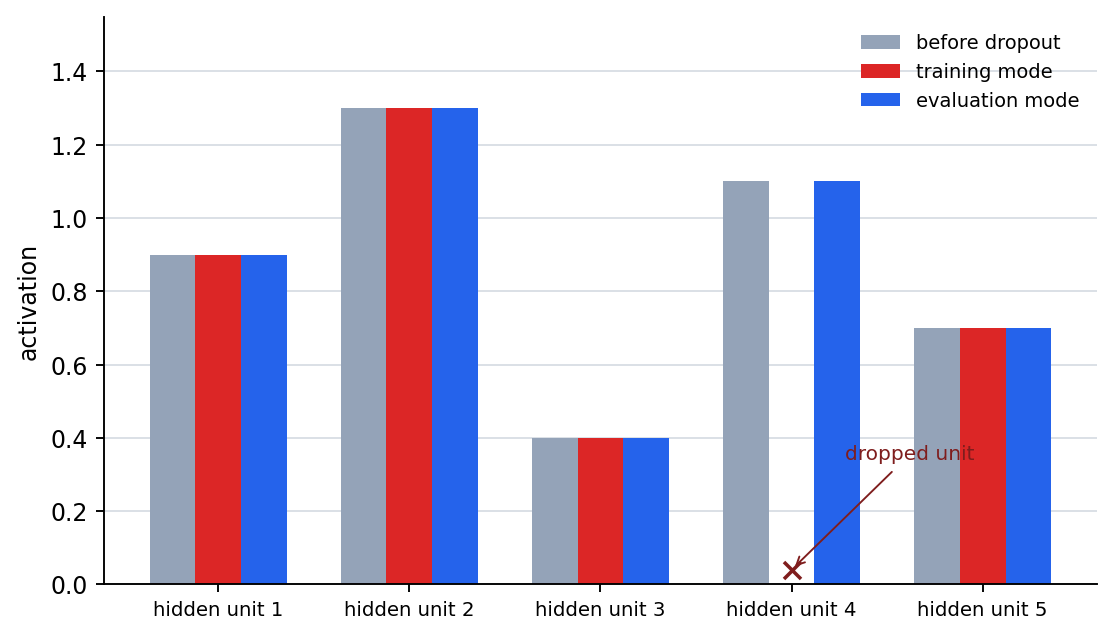
The first artifact to look at in this example is the activation value of each node in the first step. Only the fourth node, where first_step_mask is 0, is turned off in training mode, while evaluation mode keeps the original activation.
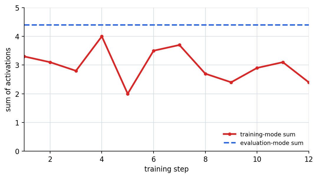
The second artifact is the sum of activations over several training steps. Here the combination of missing paths changes by step in training mode, so the sum wobbles as in train_sum_range = [2.0, 4.0], while the evaluation-mode sum stays fixed at 4.4 for the same input.
| Comparison | The key to read now |
|---|---|
before vs train | In training mode, some nodes can actually disappear at each step. |
train vs eval | Train mode shakes paths, while eval mode keeps the same input stable. |
train_sum_range | In this log example it acts as an auxiliary sign that some path combinations rested in turn. The core is not the sum itself, but the pressure that breaks path dependence. |
Even when reading the output numbers, we should separate how many became 0 from what learning pressure appears as a result.
| Comparison | What appears first in the output | Interpretation that is easy to leave if we look only at the numbers | Interpretation that changes once we include dropout |
|---|---|---|---|
before vs train | In the first step, one 1.1 disappears, and across multiple steps the resting node combination changes. | It can look as if information was simply reduced and only damage was done. | Because the remaining paths must support the output even when specific paths are missing, pressure appears that reduces shortcut dependence. |
train vs eval | For the same input, train mode shakes while eval mode keeps the original values. | It can look as if the implementation is inconsistent or unstable. | The roles are separated so that noise is deliberately added only during learning, while evaluation remains stable. |
train_sum_range vs eval_sum | In this log example the train sum wobbles by step, while the eval sum stays at its original level. | It is easy to think smaller or shakier train values simply mean worse performance. | What matters here is not the size of the sum itself, but that the model is made to learn a representation that survives even when some paths are empty. |
In other words, when reading dropout the reader should hold onto not only how many became 0, but also is the model being forced to hold up even when a specific path is missing.
The example above intentionally omitted scaling so that the path-resting intuition would appear first. But dropout in real frameworks usually uses inverted dropout, which scales the remaining activations by 1 / keep_probability. This keeps the average value scale from drifting too far away from evaluation mode even while some paths are missing during training.
The next example reads the same CSV log again, but applies inverted scaling to the values that survived in training mode. The point is not that dropout always makes values smaller, but that some paths rest while the remaining paths are rescaled so the expected train/eval scale stays closer.
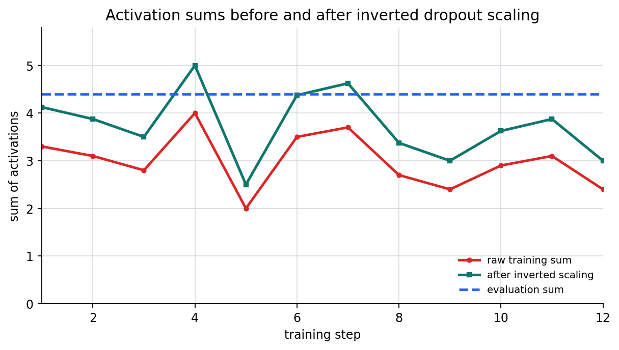
This output does not mean that adding scaling makes training mode identical to evaluation mode. The active path combination still changes when the mask changes. Inverted dropout only rescales the surviving values so that path removal during training and stable computation during evaluation do not drift too far apart in value scale.
Dropout reconnects several concepts from earlier in Part 5 at the same time.
- it prevents readers from understanding regularization from P5-8.1 only as
a penalty formula - it introduces the idea of intentionally injecting noise during learning to help generalization
- it confirms again why the difference between training mode and evaluation mode from P5-6.4 is practically necessary
Where Should We Place Dropout in the Learning Loop
Once the general viewpoint of regularization is fixed, it is natural to bring in dropout when asking is a form of overfitting control needed that cannot be explained only by a penalty. Dropout should not be read as an extra feature attached after the optimizer. It should be read as a device that temporarily lets some paths rest during the forward computation so that learning cannot depend only on a specific shortcut.
| Problem scene that appears first | Why the dropout viewpoint helps first | Where it leads next |
|---|---|---|
| it feels as if the model depends too heavily on one specific path or one hidden node | It shows the regularization intuition of shaking the structure itself so the model uses multiple paths. | In P5-8.3 we regroup it while distinguishing it from computational stabilization conditions. |
| data is limited or the fully connected layers are large, so memorization looks easy | It explains why random path removal helps suppress overfitting. | It connects back to the larger view of regularization and a reorganization of the learning loop. |
| we need to show again why the difference between training and eval mode matters in practice | Because dropout is one of the most intuitive cases that reveals the mode difference. | We look again together at the learning loop in P5-6.1 and the stabilization axis in P5-8.3. |
| explaining regularization only with penalty terms feels too narrow | It expands the idea that regularization is a design philosophy through a concrete case. | It prepares us to compare it with other regularization techniques. |
Checklist
- Can you explain that dropout is a regularization technique that reduces dependence on specific paths?
- Can you explain why dropout behaves differently in training mode and evaluation mode?
- Can you explain dropout as
regularization that temporarily lets some paths rest so that dependence on specific shortcut paths is reduced? - Can you explain that in evaluation mode the same random removal is usually not kept?
- When you need an intuitive case that shows the training/eval mode difference again, can you bring back random path removal and the evaluation-mode difference?
- Do you understand that this section plays the role of
structure-level controlin Chapter 8, and that the next section moves on tothe conditions that let deep computation actually hold up?
Sources and References
- Nitish Srivastava et al.,
Dropout: A Simple Way to Prevent Neural Networks from Overfitting, JMLR, 2014, checked on 2026-07-19. https://jmlr.org/papers/v15/srivastava14a.html - Ian Goodfellow, Yoshua Bengio, Aaron Courville,
Deep Learning, MIT Press, 2016, checked on 2026-06-29. https://www.deeplearningbook.org/ - Aurélien Géron,
Hands-On Machine Learning with Scikit-Learn, Keras, and TensorFlow, 3rd ed., O'Reilly, 2022, checked on 2026-07-19. https://www.oreilly.com/library/view/hands-on-machine-learning/9781098125967/