P5-9.1 GPUs and Parallel Processing
Section ID:
P5-9.1Version:v2026.07.26
Up through Chapter P5-8, we looked at the learning computation and regularization that happen inside deep learning models. If we widen the view a little from there, the next question appears.
Why did deep learning, which needs so many parameters and repeated computations, suddenly start to look practical only from a certain period onward?
When answering this question, it is hard to leave out the GPU (graphics processing unit) and parallel processing.
The spread of deep learning did not happen through algorithmic ideas alone. It is strongly connected to the development of computational resources that can process very large amounts of the same operation at the same time.
When the story of computational resources starts to feel abstract again, reread together the glossary entries on GPU (graphics processing unit) and parallel processing.
The Question That Connects GPUs to Parallel Processing
- Why does deep learning require so much computation?
- At the introductory level, how should we distinguish CPUs and GPUs?
- What is parallel processing, and why does it fit deep learning well?
- Why is the GPU often described as a turning point in the history of deep learning?
This section first closes why deep learning looks like a problem of repeating the same numerical operations a huge number of times, and why that repeated computation fits GPUs and parallel processing well. In other words, the focus here is on holding onto the big picture of computational resources.
At the same time, it is also clear which question will be made more concrete next. What kind of data groupings and shapes are actually fed into the deep-learning computations that GPUs handle well is explained in the next section, P5-9.2, through batches and tensor computation. Why Transformers fit GPU-style parallel processing so well is revisited later in P5-14.4.
Standards for Repeated Operations and Compute Resources
- You can explain that deep learning is sensitive to computational resources because of large matrix operations and repeated computation.
- You can explain the difference between CPUs and GPUs intuitively through
how work is grouped. - You can describe how parallel processing affected the speed and practicality of deep-learning training.
- You can read historical turning points such as AlexNet from the GPU viewpoint.
Why Does Deep Learning Require So Much Computation
Even a single prediction in a deep-learning model performs many multiplications and additions. In the training stage, loss computation, backpropagation, and optimizer updates are added on top of that.
For example:
- if the input is large
- if the hidden layers are large
- if there is a lot of data
- if we repeat many epochs
the amount of computation grows very quickly.
In deep learning, the following kinds of computation are repeated in particular.
- vector and matrix multiplication
- addition and multiplication at large tensor scales
- repeated computation at the batch level
In other words, deep learning is closer to a problem where very similar numerical operations are repeated in enormous quantity than to one single complicated problem.
How Should We Distinguish CPUs and GPUs at the Introductory Level
The following analogy is the safest one.
- a CPU is closer to a small number of strong workers handling many kinds of tasks flexibly
- a GPU is closer to a very large number of workers dividing up similar tasks and handling them at the same time
This analogy is not a perfect hardware explanation, but it is enough for explaining why deep learning fits GPUs so well.
That is:
- tasks such as operating systems, browsers, and complex condition branching feel more CPU-like
- tasks that repeat the same numerical operations in large volume feel more GPU-like
Deep learning fits the latter case very well.
What Is Parallel Processing
Parallel processing is a way of dividing up multiple computations and handling them at the same time. It is enough to understand it like this.
Rather than handling independent or similar computations one by one in a single line, we split them across several computational resources and process them simultaneously.
In deep learning, the following are especially suitable for parallelization:
- multiple samples inside one batch
- the calculation of many matrix elements
- operations across multiple channels and feature maps
That is, because deep learning repeats many numerical operations of the same pattern, it has a structure that fits GPU-style parallel processing well.
Why Do Deep Learning and Parallel Processing Fit Well Together
Deep-learning computation can mostly be summarized by the following three traits.
- it creates large matrices
- it applies the same operation at many positions
- it processes many samples at once
This structure is fairly easy to split into many separate computations.
For example:
- applying a convolution to different positions in one image
- applying the same linear layer to multiple samples in a batch
- calculating many elements of a matrix at the same time
all fit the strengths of a GPU.
Because deep learning repeats huge amounts of the same kind of numerical computation, it fits well with a style where many compute units move at the same time.
If we draw this difference by separating sequential processing and parallel processing, it looks like this.
flowchart TD
  subgraph CPU["CPU-like sequential path"]
    direction TB
    A1["Sample 1"] --> B1["Compute"]
    B1 --> C1["Sample 2"]
    C1 --> D1["Compute again"]
    D1 --> E1["Sample 3 next"]
  end

  GAP["Comparison focus: how the same work is arranged"]

  subgraph GPU["GPU-like parallel path"]
    direction TB
    subgraph INPUTS["Samples grouped at once"]
      direction LR
      A2["Sample 1"] --> A3["Sample 2"]
      A4["Sample 3"] --> A5["Sample 4"]
    end
    A2 --> P["Same matrix operation"]
    A3 --> P
    A4 --> P
    A5 --> P
    P --> O["Outputs together"]
  end

  CPU --> GAP --> GPU
The result to confirm first in this diagram is that the core of the GPU is not it performs more complicated computation, but it is easy to place the same computation across many samples and positions at once.
Why Does the GPU Look Like a Turning Point in History
The core ideas of deep learning did not suddenly appear only recently. Key concepts such as the perceptron, multilayer neural networks, and backpropagation had existed much earlier. Yet one reason deep learning spread rapidly after a certain time is that it became possible to compute it.
In particular, AlexNet in 2012 is often described as a turning point where the following elements came together.
- large-scale data (ImageNet)
- a deeper CNN structure
- GPU-based training
- the combination of training techniques and regularization techniques
So ideas alone were not enough. Computational resources that could run those ideas at real scale were needed alongside them.
Why Is AlexNet Mentioned So Often
AlexNet can be understood like this.
A representative case that made deep learning look like a real performance turning point beyond a research concept
AlexNet is mentioned so often not simply because the model was large. It is because large-scale GPU-based learning showed a major performance gap in image recognition, and the practicality of deep learning started to be widely recognized.
For that reason, the GPU looks not merely like a component, but like the device that lifted ideas into industrial-scale experiments in deep-learning history.
Cases and Examples
Case. Calculating The Same Risk Score One By One Versus Grouping It As A Batch
Suppose we compute a risk score from sensor values collected from 4 factory lines. Each line has 3 features, and we apply the same weight vector to every line. At first, people can easily feel that there is no major difference between calculating line 1 score, line 2 score, and line 3 score one after another, because the final result is the same anyway. In a small example, that is actually true. Even on a CPU, we can follow line by line how the score is created.
But the more important difference in this section is not the score itself. It is how the computation is organized. If there are not 4 lines but 4,000, and the same linear operation repeats at every learning step, then the difference between running the same computation sequentially line by line and grouping the entire batch at once immediately becomes large. The core of GPUs and parallel processing also lies here. They do not suddenly add more complicated mathematics. They create a structure in which many multiplications and additions of the same kind are stacked up and processed at the same time more easily.
So there are two results we should confirm first in this case.
- Can sample-by-sample repeated computation and batch matrix computation produce the same score?
- As the batch gets larger, how quickly does the burden of sequential repetition grow?
If this case is fixed first, it becomes more natural to understand below why the example looks at same result and scalar multiply count together.
Practice and Example
The goal of this example is to place side by side the case where the same linear operation is applied to one sample at a time and the case where it is applied to the whole batch at once.
Input:
- a small batch with 4 lines and 3 features each
- 3 weights applied in common to every line
Output:
- the risk score for each line
- the score obtained from one matrix computation
- the number of repeated computations
- a comparison of how the scale of repeated computation grows as the batch gets larger
Problem situation:
- we need to confirm directly that batch computation handles the same operation by grouping it into one matrix computation instead of repeating it once per sample
- even in a small example, if we also look at the growth in repetition count, it becomes easier to read why computational resources change what experiments are possible
Concepts to confirm:
- batch matrix computation produces many sample scores at once
- once we confirm that repeated computation and matrix computation give the same result, the meaning of batch processing becomes clearer
- we must also see that as the batch gets larger, the scale of sequential repetition grows immediately
For beginners, it is better to read this example in the following three steps.
| Reading step | What to look at first | The question to hold onto right after |
|---|---|---|
| 1 | how each line score is calculated | do sample-by-sample repeated computation and batch computation produce the same score? |
| 2 | what the scalar multiply count is | as the same operation grows with the batch, how quickly does it increase? |
| 3 | why do we talk separately about CPUs and GPUs? | even if the result is the same, does the way computation is organized change the practical range of experiments? |
Input:
We use the line batch and common weight vector summarized above.
Before reading the code, it helps to predict what will stay the same and what will grow.
| Comparison | Comparison to predict first | Reason for the prediction |
|---|---|---|
scores_one_by_one vs scores_batch | they will likely produce the same result | because the meaning of the computation is the same and only the grouping method is different |
scalar multiply count | it will likely grow immediately as the batch and feature count grow | because repeated multiplication accumulates across the number of samples and features |
| experiment burden | as the batch and model grow, CPU-style sequential computation will likely become more burdensome | because the same kind of repeated computation increases rapidly |
The difference we want to confirm here also does not end with a simple comparison of computation size. Even if the same score is obtained, the CPU-side reading should lead to how long does it take to finish this one experiment, while the GPU-side reading should lead to how many times can we change batch size, input feature count, or weight settings and try again. In other words, the computational difference in this section has to connect all the way to the difference in experiment turnaround.
The purpose of this table is to read separately that the result is the same, but the computational burden grows. This code keeps batch size and feature count directly changeable so that readers can experiment immediately with which values are more sensitive to the growth of repeated computation.
In the output, first check whether scores_one_by_one and scores_batch match, and then see at what pace the amount of computation grows when batch and feature count become larger.
- even though the content of the computation is the same, real deep-learning frameworks group such operations into
batch-wide matrix computation - even in a small example like this, the same multiplication is repeated 12 times, and as the batch or feature count grows, this repetition count grows immediately as well
- the strength of the GPU is that it can handle large volumes of these repeated multiplications and additions in parallel
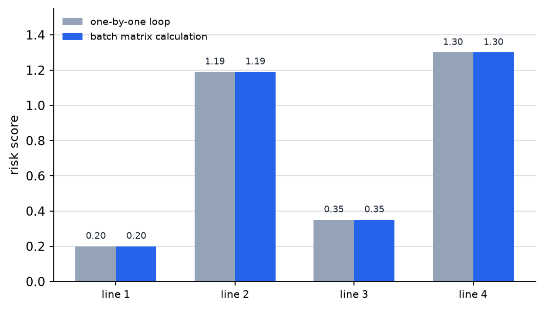
The first artifact is the line-by-line risk score. Sample-by-sample repeated computation and batch matrix computation produce the same score, but the key shown by this graph is not only the result is the same. It is the same result is obtained through different computational organization.
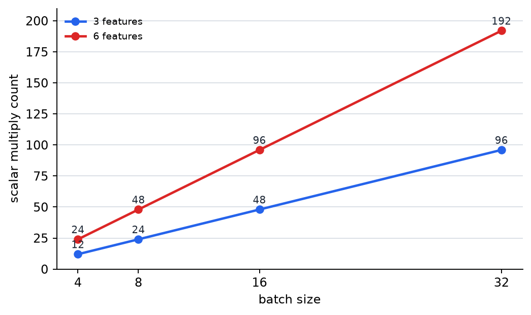
The second artifact is the rising curve of scalar multiply count. In the current example with 4 lines and 3 features, 12 multiplications are needed, but when we grow batch size and feature count together, we can read more directly how quickly repeated computations of the same kind grow.
| Comparison | The key to read now |
|---|---|
scores_one_by_one vs scores_batch | The result is the same, but the computational organization is different. |
the increase 12 -> 24 -> 48 -> 96 | As the batch and feature count grow, the burden of the same kind of multiplication grows quickly. |
| the CPU-vs-GPU intuition | The value of the GPU does not end with finishing the same computation faster. It also makes larger batches and more experiments practically possible. |
Even when reading the output numbers, we should separate did we get the same result from what scale of computation do we have to bear to get that result. For beginners, it helps to reread the output lines one by one like this.
| Output line | Meaning to read right away | Question that follows next |
|---|---|---|
same result = True | Sample-by-sample repeated computation and batch computation are mathematically doing the same thing. | Then is the real difference in how the computation is organized? |
scalar multiply count = 12 | Even in a small batch, the same multiplication is repeated many times. | When sample count, feature count, and layer count grow, how far does the repetition burden rise? |
estimated scalar multiplies when feature count = 3/6 | Not only batch size but also feature count pushes up the speed of repeated-computation growth. | Up to what input size and model width is the experiment practically feasible? |
| Comparison | What appears first in the output | Interpretation that is easy to leave if we look only at the result | Interpretation that changes once we include the GPU viewpoint |
|---|---|---|---|
scores_one_by_one vs scores_batch | The scores are exactly the same. | It is easy to think the difference in computational method does not matter. | Even when the mathematical operation is the same, how we group and process it changes practical speed and scale. |
the increase 12 -> 24 -> 48 -> 96 | As we enlarge the batch and features, the estimated repeated-computation count grows quickly. | In a small example, the numbers are simple, so it is easy to think the real burden also grows only simply. | In real models, batch size, feature width, and layer count grow together, so repeated computation soon becomes an experiment bottleneck. |
| the CPU-vs-GPU intuition | A small example is fully manageable on a CPU. | It is easy to see the GPU as only a convenience accelerator. | Computational resources are not just a speed difference. They are the condition that turns larger batches and more trials into an actually reachable work range. |
| Experiment-operation standard | Judgment that is easy to make if we read only in a CPU style | Judgment that changes once we read up through the GPU viewpoint |
|---|---|---|
| adjusting batch size | if the same score comes out, it is easy to feel there is little reason to change the batch | once we know how the repeated-computation burden grows as the batch gets larger, we start estimating first what range of experiments can be run |
| hyperparameter search | changing learning rate or model width many times can look like only a matter of spending a bit more time | once the same operations grow rapidly, we see first that the number of settings we can actually try changes depending on computational resources |
| scaling model size | it is easy to feel that increasing features or layers should only improve accuracy | in reality repeated computation and memory burden also grow together, so before expected performance we have to ask is it even runnable? |
If we turn this result into the operation of real experiments, the CPU-style reading easily flows toward if the same score comes out, the computational method difference is secondary, while the GPU-style reading asks first with what batch size and what settings can repeated experiments actually be run. The turning point to read in this section is not merely the speed difference, but this difference in the practical range of experiment design.
The reason the GPU section matters in Part 5 is not merely to add hardware knowledge. If we see deep learning only as pure mathematical theory, the explanation of why an industrial transition suddenly happened at a certain time remains empty.
This section creates the following connections.
- the vector, matrix, and NumPy computation of Part 2
- the backpropagation and optimizer of Part 5
- the large-scale LLM training and inference cost of the next parts
That is, the GPU section is the historical bridge that explains why deep learning became a large-scale computation industry.
If we pause here once and briefly fix when should we think first from the computational-resource viewpoint rather than the model-structure viewpoint, the judgment axis in later chapters becomes less shaky.
| Question to think of first | Why the GPU/parallel-processing viewpoint is needed first | What we will not go deep into yet in this section |
|---|---|---|
| why did the model suddenly become too slow? | because we first need to see whether huge amounts of the same operation are being repeated, and whether the batch and matrix computation are the bottleneck | framework kernel optimization, CUDA internals |
| do we need to run many experiments, but it takes too long? | because computational resources are not only a speed issue but the condition that makes experiment turnover itself possible | TPU, NPU, and the details of distributed-training infrastructure |
| why does the very possibility of training change as the model grows larger? | because increasing parameter count and input size together push up memory and operation limits | memory bandwidth, hardware-architecture details |
Checklist
- Can you explain why GPUs and parallel processing are strongly connected to the spread of deep learning?
- Can you describe how the development of computational resources and the development of model structure fit together?
- Can you explain that deep learning is a computational problem that repeats large-scale numerical operations?
- Can you say that GPUs are strong at handling large volumes of similar computations at the same time?
- Can you explain GPUs not only as
parts that run deep learning faster, but asthe condition that lifts large-scale repeated computation into a practical experimental scale? - Can you explain that even though the same score can be obtained through both sample-by-sample repeated computation and batch matrix computation, the computational organization changes the practical range of experiments?
- When execution speed and experiment turnover look like a bigger bottleneck than model structure, can you think first of the computational-resource viewpoint?
- Do you know that AlexNet is often read as a turning point where data, model, GPU, and training techniques were combined?
Sources and References
- Alex Krizhevsky, Ilya Sutskever, Geoffrey E. Hinton,
ImageNet Classification with Deep Convolutional Neural Networks, NeurIPS 2012, checked on 2026-06-29. - Ian Goodfellow, Yoshua Bengio, Aaron Courville,
Deep Learning, MIT Press, 2016, checked on 2026-06-29. https://www.deeplearningbook.org/ - NVIDIA,
What Is a GPU?, NVIDIA Docs / corporate documentation, checked on 2026-06-29. https://www.nvidia.com/en-us/glossary/gpu/