P5-11.1 The Intuition of Convolutional Neural Networks (CNNs)
Section ID:
P5-11.1Version:v2026.07.26
In Chapter P5-10, we saw that deep neural networks can learn more useful representations as they pass through layers. If we now narrow that viewpoint to images, the next question appears.
For data with spatial structure such as images, why do we say a convolutional neural network (CNN) is more natural than an ordinary fully connected layer?
The structure that answers this question is the convolutional neural network.
A convolutional neural network is a neural network that does not look at the whole image in one identical way at once, but instead repeatedly inspects small local patterns and learns larger visual structures from them.
When you need to reset the basic definition for reading image structure, return to the glossary entry on CNN (convolutional neural network).
The Question of Why CNNs Fit Images
- Why does a CNN fit images well?
- What does it mean to look at local patterns?
- What is different from using only fully connected layers?
- Why is a CNN important from the viewpoint of representation learning?
The key that has to be closed first in this section is that because images create meaning through nearby positions together, a structure is needed that repeatedly reads local patterns.
That is, the handle of this chapter changes from shall we mix the whole image at once to shall we repeatedly read the local structure of nearby positions.
What we read first here is not a learning procedure such as the optimizer or regularization, but the input structure: in what order and over what range do we group nearby clues and lift them into larger visual structure.
| What we read in this section | What we hand off to the next section or supplementary reading |
|---|---|
| why the local structure of images has to be read repeatedly | how convolution and pooling actually compute that structure |
| the difference in how fully connected layers and CNNs look at the input | by what standard we compare later vision structures after CNNs |
The concrete operations of convolution and pooling are handled next in P5-11.2, and the larger flow of representation learning in the image domain was already fixed in P5-10.1 and P5-10.2. In this section, we reread that larger flow on top of image scenes. A broader comparison of vision structures after CNNs continues in supplementary reading P5-11.3 at the level of by what viewpoint should we compare CNNs and Vision Transformers (ViT).
Standards for Local Patterns and Shared Filters
- You can explain a CNN as
a neural network that repeatedly reads the local structure of images. - You can say why position and nearby patterns matter in images.
- You can compare fully connected layers and CNNs at the introductory level.
- Through an executable Python example, you can confirm the intuition of reading local patterns.
Why Is Spatial Structure Important in Images
An image is not just a list of numbers. Each pixel creates meaning together with the surrounding pixels.
For example:
- an edge appears from a neighboring brightness change
- a corner appears from the meeting of multiple edges
- partial structures such as valves, warning lights, and small cracks are also revealed through combinations of nearby pixels
That is, in images the relation among nearby positions is very important.
The core point is that an image is data where not only the values themselves, but also the positions of those values and how they connect to nearby values, must be read together.
In images, it is not only important that a value exists, but also where that value is and how it connects to its surroundings.
Why Is It Awkward to Use Only Fully Connected Layers
In theory, we can flatten an image into a long vector and feed it into fully connected layers. But this way does not preserve the spatial structure of the image in an intuitive way for the reader.
For example:
- it cannot naturally emphasize the relationships of neighboring pixels
- the intuition that the same pattern repeats at different positions becomes weaker
- the number of parameters can also become very large
That is, a fully connected layer is closer to mixing all inputs at once, and it is less natural for first looking at the local structure of an image.
If we compare the same difference very briefly in a table, it becomes the following.
| Viewpoint | Use only fully connected layers | CNN |
|---|---|---|
| how the input is read | flatten and read the whole thing at once | read small local regions repeatedly |
| position intuition | the intuition of neighboring pixels tends to weaken | nearby-pixel relations are read more naturally |
| reuse of the same pattern | can feel like separate learning at each position | the same filter is repeatedly applied at many positions |
| beginner-level intuition | mix all values at once | rise from small patterns to larger structure |
If we split the same image scene across the two structures, the difference becomes more direct.
| The same scene | What is easy to leave when we first read with fully connected layers | What is held onto more when we first read with a CNN |
|---|---|---|
| image of a pressure gauge dial | the overall impression of one round gauge | local clues such as needle angle, scale crossing, and boundary of the dial face |
| equipment photo | the overall color and shape impression of the whole photo | repeated partial structures such as valves, warning lights, and tank boundaries |
| surface-inspection image | the whole product silhouette and average brightness | local anomalies such as small scratches, cracks, and stains |
What Does a CNN Do Differently
A CNN does not look at the whole image all at once. Instead, it moves a small window or filter and repeatedly finds local patterns.
For example, one filter can:
- react to vertical edges
- another filter can react to horizontal edges
- and another filter can react to more complex small shapes
The important point is that this filter is not used at only one position in the image. It is repeatedly applied at many positions.
That is, a CNN can be read as a structure designed so that the same pattern can be seen similarly wherever it appears in the image.
If We First Look Through Pictures
Gauge reading and object detection are representative scenes often used to explain the intuition of a CNN. In both cases, the model does not know this is the state of the gauge or this is the object all at once from the beginning. Instead, it first reads small lines, boundaries, corners, and partial shapes, and then lifts those combinations toward a larger judgment.
If we first place side by side image scene -> clues seen first by a person -> representation built by a CNN, it becomes the following.
| Scene | Clues first seen by a person | Representation built up by the CNN |
|---|---|---|
| pressure-gauge dial image | short needle line, scale intersections, circular boundary | needle edges -> dial parts -> gauge-state pattern |
| equipment photo | valve outline, warning-light boundary, handle shape | edges/textures -> parts -> equipment-like region |
The three diagrams below show, step by step, how channel combination and hierarchical representation grow larger. The numbers and arrays are not copied from an outside figure. They are newly simplified examples created only to explain the concept.
- We first see that one filter does not discard RGB channels separately, but reads them together.
- We then see that, even for the same photo, deeper layers look at wider areas together.
- We then see how that widened field of view combines into larger visual clues over the feature map.
Figure 1. One Filter Reads The Channels Together
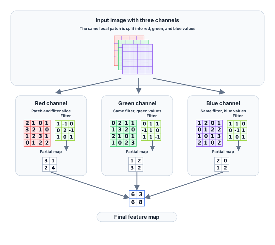
The first thing to see in this figure is not if there are three channels, the CNN processes the image as three completely separate things, but rather one filter reads same-position patches across the channels together and combines those responses into one feature map. Color information is also read together inside the local pattern, and in the end it is organized into a response map that asks what pattern appeared strongly at this position.
When reading this figure, the following order is enough.
- See that the input patch at the top is split into red, green, and blue values.
- See that one partial response map comes out of each channel.
- See that at the bottom those responses are added together into one final feature map.
That is, the core of this figure is not the final maps remain separate for each channel, but the channel-wise responses to the same-position patch combine into one pattern response.
Figure 2. Deeper Layers See More Broadly
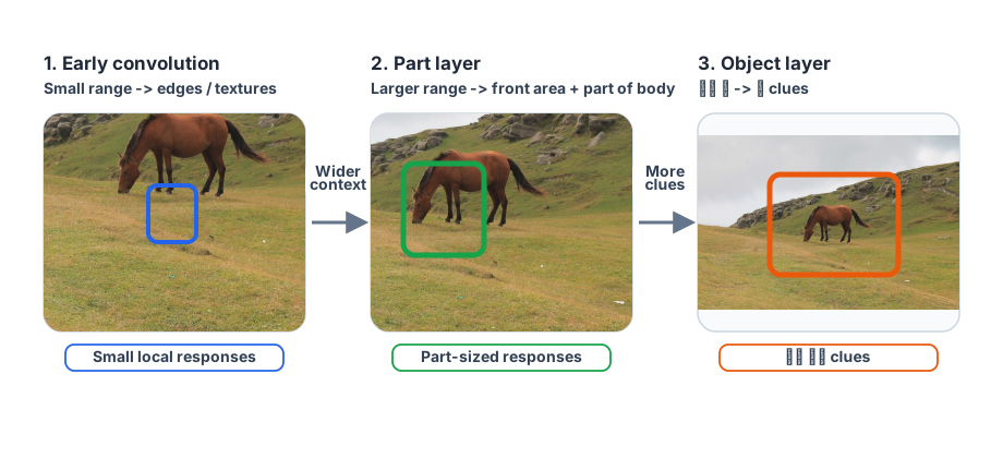
The second figure reuses the same equipment photo three times and isolates only the point that the input photo stays the same, but the receptive field widens as the layer gets deeper. The left panel is the situation where early convolution reads local clues such as metal texture and valve boundaries in a small local patch. The middle panel is the situation where a wider area is read together so that grouped partial structures such as pipe junctions and the upper part of the tank can be read. The right panel is the situation where many part clues are gathered together so that clues at the level of the overall equipment body can be read.
What is especially important in this figure is that the photo itself does not change. What changes is not the input photo, but the range one layer can read together and the size of the patterns it can group inside that range.
Figure 3. Reaction Maps Also Combine Into Larger Clues
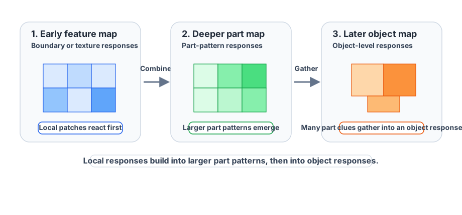
The third figure now shifts attention from the photo to the response maps. In the early feature map, responses to edges or textures at specific positions become strong first. In a deeper part map, a larger part pattern appears more stably when nearby responses line up together. In a later object map, object-level activation becomes possible when multiple part clues align together.
That is, in explaining a CNN, the important point is not did it memorize the whole photo at once, but do early convolution responses actually accumulate into larger object clues through the feature map. This third figure shows that accumulation again from the viewpoint of the response map.
If we reduce a pressure-gauge dial image into a very simple black-and-white scene, we can think of it as follows.
| gauge-like image patch | what stands out first |
|---|---|
[[0, 1, 1, 0], [0, 1, 0, 0], [1, 1, 0, 0], [0, 0, 0, 0]] | a thin needle line, intersection with the scale, possible circular boundary |
In an equipment scene too, the early clues first appear as local responses such as valve boundaries, tank outlines, and warning-light shapes.
| equipment-like image patch | what stands out first |
|---|---|
[[pipe, pipe, tank, tank], [valve, tank, beacon, beacon], [valve, tank, tank, panel]] | valve boundary, long tank body, rectangular control-box outline |
These two tables do not literally draw a real high-resolution image, but they show that the first question to hold onto in explaining a CNN is which small part stands out first in this scene.
Even in reading a pressure gauge, the image is not first read directly as labels such as safe zone and warning zone. Rather, local clues such as the needle line, scale crossing, and circular boundary first accumulate and then rise into the gauge-state judgment.
Object detection can also be read as a flow in which local clues gather into location and label judgment for an object.
flowchart TD
  A["image pixels"]
  B["edges / textures"]
  C["wheel / window / handle"]
  D["car-like region"]
  E["object box + label"]

  A --> B
  B --> C
  C --> D
  D --> E
The result to confirm in this diagram is that object detection also is not a matter of memorizing the whole scene at once, but rather of first reading partial clues such as the valve or warning light seen in the earlier scene table, letting them gather into an equipment-like region, and then moving on to the final location and label judgment.
It Goes from Local Patterns to Larger Structure
The intuition of a CNN also naturally connects to the hierarchical representation learning that we already saw in Part 5.
- early layers: small local patterns
- middle layers: partial structures
- deeper layers: larger object clues
That is, a CNN does not connect the pixels themselves directly to the answer. It creates a hierarchical structure that rises from small local patterns toward larger visual clues, like edge -> partial structure -> object clue. So a CNN is better read not as a mere image-specific operation, but as a structure that stacks local patterns into larger visual representations.
Why Did a CNN Look Like a Turning Point
The reason CNNs drew so much attention in deep-learning history is that they showed cases in image recognition where the model learned stronger hierarchical representations than features people had built directly.
In particular, after AlexNet, CNNs showed all of the following together.
- deep neural networks can actually produce strong performance on images
- scale can be enlarged by combining them with GPU training
- representation learning can greatly replace manual feature design
That is, CNNs are one of the structures that showed the viewpoint of deep-learning representation learning most impressively in the image domain.
Cases and Examples
Representative Case. Reading A Pressure-Gauge Dial
Suppose a field camera reads a pressure-gauge dial. At first, people can easily feel that they see only the overall impression of one circular gauge, so the states can seem similar. But in actual discrimination, we have to look again at small differences such as near which mark the needle tip lies, at what angle the needle line meets the scale, and whether the circular boundary and the position of the dial face remain stable even when part of it is hidden by reflection. A CNN fits well with a way of first reading these local structures and then gradually connecting their combination to a larger representation of the gauge state.
So the result to confirm in this case is whether, rather than the overall impression of one circular gauge, local clues such as the needle tip and scale crossing actually come alive first and split the safe zone and warning zone more stably.
| Standard that is easy for a person to see first | Standard to reread from the CNN viewpoint |
|---|---|
| looking only at the overall impression of one circular gauge makes states feel similar | we must check whether small differences such as needle-tip position and scale crossing split first |
| when reflection or shadow exists, people try to judge roughly from the overall impression of the gauge | we have to read first which local clue actually makes a different response |
| because both are circular and the dial face looks similar, confusion feels natural | a CNN first sees local differences such as needle line, scale boundary, and crossing position rather than the overall circle |
The same viewpoint applies to other image problems as well. But the core to hold onto in this section is not the domain name, but which local clue comes alive before the whole impression.
If we place the three cases together, it becomes clearer why CNNs should be read not merely as an image-model name, but as a way of reading local structure before the whole impression.
| Scene | Result that is easy for a person to see first | What actually needs to be distinguished from the CNN viewpoint | What to check next right away |
|---|---|---|---|
| reading a pressure-gauge dial | it looks like one circular gauge, so the states look similar | local differences such as needle-tip position, scale crossing, and response near the boundary must come alive first | check whether the safe zone and warning zone split more stably according to local clues |
| reidentifying an equipment scene | if the whole impression of the equipment looks similar, it feels like the same scene | local structure around valves, pipes, and warning lights can be a more stable clue than lighting and background | check whether judgment of the same equipment scene remains more stable when local clues are preserved |
| industrial vision | if the overall product shape looks similar, the state looks similar | small scratches, cracks, and stain locations must split defect candidates before the overall impression | check which patch remains as the higher reinspection candidate |
Practice and Example
The goal of this example is to confirm, not by looking at the whole image at once, but by looking at small regions, which position becomes the candidate to inspect again in operation. It does not stop at extracting a few patches. It also compares a normal panel and a scratched panel side by side to show how the local response differs.
Before reading the example, the minimum points that actually need to be confirmed in this section can be fixed as follows.
| Checkpoint | Value to see directly in the example | Why it matters |
|---|---|---|
| how many local windows are created | number of 2x2 patches | because it shows that a CNN repeatedly reads many local regions rather than the whole image at once |
| how the responses split between a normal panel and a defect panel | normal best, scratch best | because even within the same product family image, once a local defect appears we can directly see at which position the response becomes larger |
| which position becomes the candidate to inspect again in operation | best patch position, score gap | because in defect inspection, which small region should be looked at again matters more than the whole average |
| why the defect panel has higher priority even when the normal panel also has some response | normal best score, scratch best score | because both can have local responses, but the defect scene can reveal a much larger local change |
Input:
- a 5x5 brightness array for a normal panel
- a 5x5 brightness array for a scratched panel
- a small window of size 2x2
Output:
- the number of possible 2x2 local patches
- the strongest local-response position in the normal and defect panels
- a simple local score at each position
- the score gap between the normal and defect scenes
Problem situation:
- in surface-inspection operations, what matters more than the overall impression of the product is
which small position becomes a candidate for reinspection, so we need to directly confirm the CNN intuition of local reading in that scene
Concepts to confirm:
- convolution creates responses by repeatedly scanning local patches
- even if scenes look like the same product, once a local defect appears the response at a specific position can become larger
- in operation, what matters more than
is the whole average differentiswhich patch becomes the candidate to look at again
For beginners, it is better to read this example in the following three steps.
| Reading step | What to look at first | The question to hold onto right after |
|---|---|---|
| 1 | normal_best, scratch_best | at what position does the normal scene and the defect scene first respond most strongly? |
| 2 | number of 2x2 patches, score gap | even in the same scene, why does a local candidate score matter more than the whole impression? |
| 3 | the two response maps | where does the local anomaly candidate come alive, and how clear is that difference? |
Input:
We use the normal panel, scratched panel, and 2x2 window summarized above.
Before reading the code, it helps to predict what comparisons will occur first.
| Comparison | Change to predict first | Reason for the prediction |
|---|---|---|
normal best score | it may be small, but likely not 0 | because even in a normal panel there can be weak local differences near the boundary |
scratch best score | it may jump much larger | because at the scratched position the local brightness change is sharper |
score gap | it will likely be positive | because in operation the candidate that needs to be looked at again can appear with a stronger response on the defect side than on the normal side |
The purpose of this table is to read first not is there a response or not, but in which scene does the stronger local response jump out.
In the output, look in order at the strongest-response position in the normal panel, the strongest-response position in the defect panel, and then the score gap between the two scenes.
The core points to confirm in this example are the following.
- a CNN does not see the whole image only once at once, but repeatedly reads small local windows
- when we compare the normal scene and the defect scene, the response score can become larger where a local anomaly exists
- in operation, the intuition of
leave the region with the largest response as the candidate to inspect againmatters - that kind of local information can later accumulate into larger representations
If we view the local response as a 4x4 map, the normal panel has several weak responses, but overall there is no large difference.
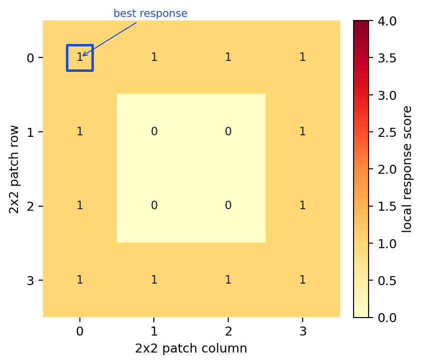
In the scratched panel, the response at a specific position jumps much larger, so the candidate position that should be looked at again becomes clearer. This difference is why a CNN should be understood as a structure that repeatedly reads local patterns rather than the overall image impression.
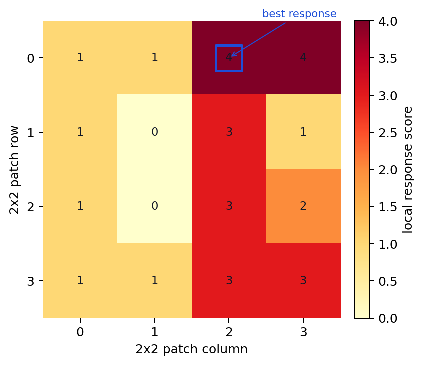
| Comparison | The key to read now |
|---|---|
normal best | Even in a normal scene, weak local responses can exist. |
scratch best | In the defect scene, a much larger response jumps at one specific patch and becomes the operational priority. |
inspection_priority | The CNN intuition puts forward not the whole photo impression, but which small region should be rechecked first. |
Even when reading the output numbers, we should separate is there any response from which region becomes the priority candidate first.
| Comparison | What appears first in the output | Interpretation that is easy to leave if we look only at the score | Interpretation that changes once we include the CNN viewpoint |
|---|---|---|---|
normal best | Even the normal panel produces a best response score of 1.0. | It can look as though the CNN cannot really distinguish because a normal scene also has some response. | Local responses themselves can exist in the normal scene too, but their size and position do not form as strong a reinspection candidate as in the defect scene. |
scratch best | The scratched panel's strongest response jumps up to 4.0. | It is easy to think the number simply got larger. | At the position with a local defect, the local response becomes much larger, showing that the CNN reveals a small anomaly location before the whole-image impression. |
inspection_priority | The final inspection priority becomes scratch panel. | It is easy to think it merely chose the brighter side. | The key is that rather than the overall average, it first chooses which 2x2 patch should be rechecked. |
That is, this example shows the operational intuition that even if the whole product photo looks similar, if the response of a patch near one corner suddenly becomes larger, it should be reviewed again. A CNN matters not simply because it classifies images well, but because it is a structure that reveals such local defect candidates before the whole impression.
CNNs are almost always treated as an important turning point in an introductory deep-learning curriculum. The reason is simple.
- they show most intuitively in the image domain what representation learning and hierarchical representation from P5-10.1 and P5-10.2 actually mean
- they explain what kind of performance transition was created by combining GPUs and large-scale data
- and they become an important comparison standard when later learning structures such as vision transformers
That is, CNNs are the chapter where the history, structure, and practicality of deep learning meet.
If we pause here once and briefly fix when should we read an image-classification problem first from the viewpoint of local patterns rather than the whole impression, the baseline for the structure explanation will shake less when moving into the next convolution section.
| Question to think of first | Why the CNN intuition is needed first | What the next section continues from here |
|---|---|---|
| why should the same object still be read similarly even if the position or background changes? | because it is more natural to read repeated local patterns at many positions than to mix everything at once | how convolution actually computes location-wise responses |
| why is the fully connected intuition weak when small scratches or partial structures matter? | because local clues have to come alive before the whole impression | what signal feature maps and pooling leave behind |
| why do CNNs appear so often as the representative structure of representation learning? | because they most intuitively show the process in which local clues accumulate into larger visual representations | the actual computational flow of hierarchical visual representation |
Checklist
- Can you explain why a CNN is natural for data with spatial structure such as images?
- Can you explain the difference between how fully connected layers and CNNs read the input?
- Can you explain that a CNN is a neural network that repeatedly reads local patterns in images?
- Can you explain an image not only as
all of the pixel numbers, but first aslocal structure created by nearby positions together? - Can you say that in images, not only the values but also the positions and neighboring relations matter?
- Can you explain that in the gauge, equipment-scene, and industrial-vision cases, the first thing to read in common is the local clue?
- When you are explaining an image problem only through the whole impression, can you think first of the viewpoint of local patterns?
- When reading convolution in the next section, are you ready to think first of
how strongly does it respond to which local pattern?
Sources and References
- Yann LeCun et al.,
Gradient-Based Learning Applied to Document Recognition, Proceedings of the IEEE, 1998, checked on 2026-07-19. https://doi.org/10.1109/5.726791 - Alex Krizhevsky, Ilya Sutskever, Geoffrey E. Hinton,
ImageNet Classification with Deep Convolutional Neural Networks, NeurIPS 2012, checked on 2026-07-19. https://papers.nips.cc/paper/2012/hash/c399862d3b9d6b76c8436e924a68c45b-Abstract.html - Ian Goodfellow, Yoshua Bengio, Aaron Courville,
Deep Learning, MIT Press, 2016, checked on 2026-06-29. https://www.deeplearningbook.org/