P5-11.2 Convolution And Pooling¶

Section ID: P5-11.2 Version: v2026.07.20

In P5-11.1, we explained a CNN as a neural network that repeatedly reads local patterns in images. The next question remains.

What is the core operation that actually computes those local patterns, and why does pooling so often appear together with it?

Convolution is the operation that computes local-pattern scores with a small filter, and pooling is the operation that organizes those results into a smaller, more summarized form.

When the operation names become mixed up again, it is useful to reread together the glossary entries on convolution and pooling.

Questions Closed By Convolution And Pooling¶

• What does convolution compute?
• What do filter and feature map mean?
• Why is pooling used, and what does it reduce?
• When the two operations appear together, how should we read the representation flow of a CNN?

This section focuses not on proving the convolution formula rigorously, but on first closing the flow in which a CNN scores local patterns and then summarizes those responses.

At the same time, it is clear what we will not widen immediately in this section. A broader comparison of vision structures after CNNs is revisited in supplementary reading P5-11.3 around CNN and Vision Transformer (ViT). Padding, stride, and dilation are handled only as much as needed here to understand how the filter reads the input.

Standards For Reading Local Responses And Summaries¶

• You can explain convolution as the operation where a small filter computes local-pattern scores.
• You can explain a feature map as the spatial record of filter responses.
• You can say why pooling is used to reduce spatial size and summarize important responses.
• Through an executable Python example, you can confirm the intuition of convolution and max pooling.

From Filter Responses To Pooling Summaries¶

1. First look at how convolution computes local-pattern scores.
2. Then look at how the result remains as a response map called a feature map.
3. Then look at how pooling passes that response onward in a smaller and more summarized form.
4. Then organize how convolution and pooling connect into one flow.
5. Finally look again at how padding, stride, and dilation change the way this flow is read.

What Does Convolution Do¶

Convolution moves a small filter across many positions in the image and scores how well each position matches a certain pattern.

The core point is that the filter carries the small pattern it wants to find and sweeps across the image to produce response scores.

• the filter can be seen like a small pattern template to find
• it performs multiplications and additions with each local patch of the image
• and produces a response score for that position

That is, convolution does not judge the whole image at once. It is a way of repeatedly applying a small pattern detector to the full set of positions.

What Does A Filter Mean¶

A filter is usually a small array of numbers. For example, a 3x3 filter can look at a 3x3 local patch.

A filter is a small bundle of weights that is learned to respond to patterns such as edges, directions, textures, or small shapes.

As a CNN is trained, these filter values also change to fit the data. That is, a person does not directly design every filter. The model also learns which filters are useful.

What Is A Feature Map¶

If one filter is applied across the whole image, the result is a new 2D array that stores how strongly that filter reacted at each position. This is called a feature map.

That is:

• over the input image
• the filter is applied at each position
• and the recorded response values become

the feature map.

The key point is that a feature map is the result that records, by position, where and how strongly one specific filter reacted in the image.

A feature map is a map that records where in the image, and how strongly, a specific filter reacted.

At this point it helps readers to fix the following distinction together.

Why Is Pooling Needed¶

If we only keep stacking convolution results as they are, the spatial size can remain large and the amount of computation can also become large. It is also not always best to keep carrying every bit of detailed position information all the way to the end.

Pooling plays the role of reducing such information into a more summarized form.

For example, max pooling leaves only the largest response inside a small region.

Pooling reduces some detailed position information, but passes important responses onward in a more compressed way.

Why Is Max Pooling Intuitive¶

Max pooling chooses one largest value inside a small window. This gives the reader the following intuition.

• it keeps the strongest pattern response in that region
• it can become less sensitive to small position changes
• it compresses the computation by reducing spatial size

That is, max pooling is best read as a summary that keeps the most noticeable signal.

If we compare this difference more briefly, it becomes the following.

If we split the same image scene into those two stages, the difference becomes more direct.

How Should We Read Convolution And Pooling Together¶

If we connect them in a very simple form, it looks like this.

flowchart TD
  A["input image"]
  B["convolution<br/>detect local pattern"]
  C["feature map"]
  D["pooling<br/>summarize response"]
  E["smaller feature map"]

  A --> B
  B --> C
  C --> D
  D --> E

This diagram shows the three actions find -> record -> summarize.

1. Convolution first finds a local pattern.
2. The feature map records that response by position.
3. Pooling passes that record on in a smaller and more summarized form.

This flow is easier to read when we place a practical inspection scene and a numeric array side by side. The example below simplifies a small sealing patch where the left-right column heat distribution changes sharply at the sealing edge.

Now suppose we place a 2x2 filter that reacts to left-right column differences over this input.

If we move the filter one step at a time and compute, the following feature map appears.

If we divide the same transform into one step at a time, it can be read as follows.

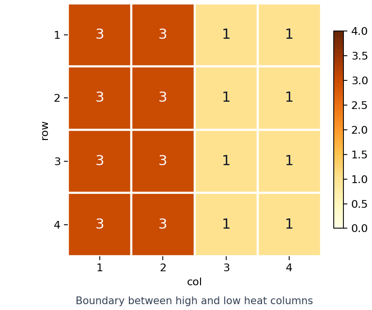
The input patch is still closer to the small heat-distribution scene seen by a person. High values on the left and low values on the right are placed together, but at this stage where is the boundary has not yet been separated into a score.

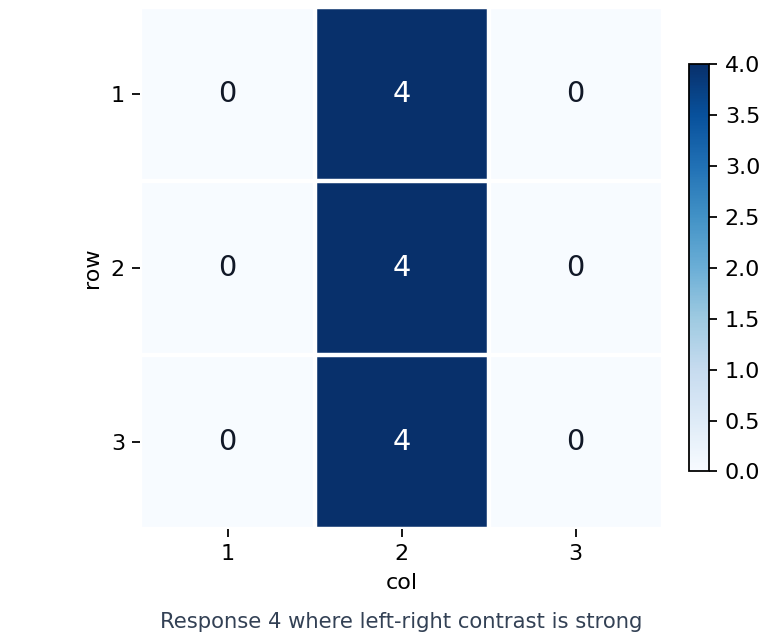
After convolution, it becomes a response map showing how well each position matches the filter. Here, the value 4 repeats only at the middle position where the left-right column difference actually appears, meaning the input scene has turned into a position map of boundary responses.

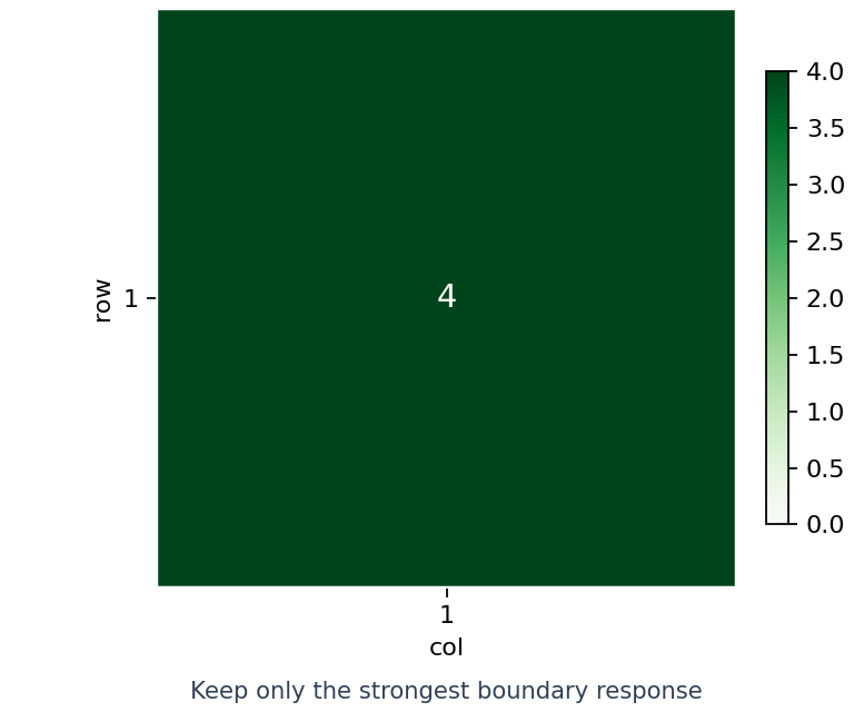
Max pooling does not pass that whole response map onward as-is. Instead, it keeps only the strongest response inside the small region. What changes at this stage is that rather than the detailed position, the summary signal there was a strong sealing-boundary change in this region is passed to the next layer.

The key to reading these numbers is the following.

• 0 means a position where the left-right difference expected by the filter is almost absent
• 4 means a position where the heat-distribution boundary the filter wanted was captured strongly
• [[4]] after max pooling means that even if detailed position is reduced, the key point there was a region with a strong sealing-boundary change remains

That is, the small inspection patch holds onto the human scene, while the sample matrices show what kind of numeric summary convolution and pooling actually produce.

This flow shows that a CNN:

• first finds a pattern
• then records that response
• then passes it on to the next layer in a more compressed form

That is, convolution scores local patterns, and pooling passes those scores onward in a smaller form that the next layer can read more easily.

Before moving to the next ViT comparison section from here, if we fix once more what unit a CNN actually uses for computation, it can be seen as follows.

flowchart TD
  A["same equipment image"]
  B["small local windows slide with overlap"]
  C["compute a local response score at each position"]
  D["strong responses are recorded in the feature map"]
  E["baseline for the next layer to read larger structure"]

  A --> B --> C --> D --> E

The points to hold onto first in this baseline diagram are the following.

• the first computation unit of a CNN is not the whole image, but a small local window that moves with overlap
• what each window first produces is a local response score to the question how well does this position match the filter pattern
• so when we later look at ViT patch tokens, we can compare a method that sweeps over small windows and a method that reads already cut patches on the same input

If we read CNN only as a past structure that existed before Part 5 or before Transformers, it is easy for it to look like an old model name for images. But in Part 5, the responsibility of the CNN is already closed here. That is, the CNN is a structure that has its own answer to how should we detect and summarize local patterns in images, and the later parts only need to continue by handling different data-structure problems, not by replacing this answer.

What Do Padding, Stride, And Dilation Mean¶

Although convolution and pooling are the center of this section, it is still better to fix at least the minimum meaning of padding, stride, and dilation, whose names already appeared above.

All three adjust how the filter reads across the input.

The differences among the three are the following.

• padding is the choice to add margins outside the edges
• stride is the choice to determine the step size of the filter movement
• dilation is the choice to widen the spacing between cells inside the filter

If we compress this into three ways of reading the same input, it becomes the following.

flowchart TD
  A["Same input image"]

  subgraph P["Padding"]
    P1["Add border space"]
    P2["Keep edge regions visible longer"]
  end

  subgraph S["Stride"]
    S1["Move filter by larger steps"]
    S2["Reduce output size faster"]
  end

  subgraph D["Dilation"]
    D1["Spread filter intervals"]
    D2["See a wider area without a bigger kernel"]
  end

  A --> P1
  P1 --> P2
  A --> S1
  S1 --> S2
  A --> D1
  D1 --> D2

The result to confirm first in this diagram is that all three change not what the filter is trying to find, but how it sweeps across the input.

This section does not unfold the three terms into formulas, but when reading the convolution explanation below, it is enough first to hold onto them as devices that adjust the content of the filter, the movement of the filter, and the range the filter covers. The small scene below shows that difference directly.

First imagine that we are reading the same 1D line.

1
2

input = [A B C D E]
filter size = 3

At that point, the three terms answer different questions.

• padding: shall we put margins at both ends?
• stride: how many cells shall we move at a time?
• dilation: shall we read the filter cells right next to one another, or with gaps between them?

That is, all three are choices that change how we sweep, rather than changing convolution itself.

Why Is Padding Needed¶

Without padding, the filter cannot go outside the edges of the input, so information near the boundary is relatively easy to read less often.

For example, if we move a 3x3 filter over a 5x5 image as-is, the filter center moves stably only in the inner region rather than on the outer border. In that case, a small line or corner on the border can be reflected less.

Padding is the way of placing one more margin around that outside.

• without a margin, it ends immediately at the border
• with a margin, positions near the border get one more chance to be read

That is, padding creates one more chance to read near the border so that edge information is not lost too quickly.

Written with a very short line example, it becomes:

1
2

without padding: [A B C] [B C D] [C D E]
with padding:    [0 A B] [A B C] [B C D] [C D E] [D E 0]

The key here is that the border also gets a chance to be computed.

What Does Stride Change¶

Stride determines how many cells the filter moves at once.

Seen very simply:

• if stride is 1, it moves one cell at a time and reads densely
• if stride is 2, it jumps two cells at a time and reads more coarsely

For example, if a filter of width 2 reads across a line of length 4:

• with stride 1 it reads with overlap like [1-2], [2-3], [3-4]
• with stride 2 it jumps more broadly like [1-2], [3-4]

That is, stride is the choice that decides how densely shall we sweep. As stride grows, the output size shrinks faster and the computation is summarized more coarsely.

If we reread this in terms of images:

• stride 1: we look at almost every position without skipping
• stride 2: we do not look one by one, but more sparsely

That is, if stride grows, the output shrinks faster, but detailed position differences are seen less.

Why Does Dilation Have Its Own Name¶

Dilation widens the spacing between filter cells so that a wider range can be seen without making the filter itself larger.

For example, if we place a 3-cell filter normally, it reads directly neighboring cells. But if dilation is added, it can read positions farther apart together, like first cell, a cell after skipping one, another cell after skipping one more.

That is, dilation is:

• a choice that does not greatly increase the number of parameters
• used when we want to see a wider receptive field
• by widening the spacing between cells inside the filter

So dilation is the choice that lets the filter see a wider receptive field by widening the spacing inside it without greatly increasing the number of parameters.

Seen with a 1D line example, the difference becomes even simpler.

1
2

without dilation: [A B C]
with dilation:    reads separated positions together like [A _ C _ E]

That is, the number of filter cells stays the same, but only the range seen at once becomes wider.

If we regroup the three terms again in one line, it becomes the following.

At the introductory stage, it is enough to recheck them through the following questions.

• padding: do we want to let the border be read more too?
• stride: shall we read more densely, or jump farther?
• dilation: do we want to see a wider range without increasing the filter size?

If We Look At All Three Differences Together Through A Small Numeric Example¶

If we only talk about them in words, the three terms can feel similar, so let us regroup them again through a scene where the same 3x3 filter reads a very small 5x5 input.

 1
 2
 3
 4
 5
 6
 7
 8
 9
10
11

input
1 0 0 0 1
0 1 0 1 0
0 0 1 0 0
0 1 0 1 0
1 0 0 0 1

filter
1 0 1
0 1 0
1 0 1

At this point, what the reader should look at first is not the filter values themselves, but what position grouping is read at once.

That is, all three settings are devices that change not what the filter finds, but with what interval and over what range the filter moves.

A Small Example For First Seeing The Difference In Settings¶

The goal of this small example is to confirm with our eyes how padding, stride, and dilation change the output size and the region actually read. The goal is not to memorize every convolution value, but to hold onto that even with the same filter, if the scanning method changes, the output shape and the patch being read change together.

Before reading the code, if we look in order at the following three values first, the structural difference in this section spreads less.

Input:

• a 5x5 sealing-inspection patch
• a 3x3 filter
• different padding, stride, and dilation settings

Output:

• the shape of the output matrix for each setting
• the patch actually read at the first position
• the convolution result for each setting

Problem situation:

• although the names padding, stride, and dilation sound similar, they make the filter read the image range differently

Concepts to confirm:

• convolution settings change both the result shape and the actual patch range
• when we look at the first-position patch together with the final result, the difference of each setting becomes more visible

Input:

We use the input image, filter, and several padding, stride, and dilation settings summarized above.

 1
 2
 3
 4
 5
 6
 7
 8
 9
10
11
12
13
14
15
16
17
18
19
20
21
22
23
24
25
26
27
28
29
30
31
32
33
34
35
36
37
38
39
40
41
42
43
44
45
46
47
48
49
50
51
52
53
54
55
56
57
58
59
60
61
62

# This example compares how padding, stride, and dilation change convolution output shape, the first patch, and result values.
import numpy as np

image = np.array([
    [1, 0, 0, 0, 1],
    [0, 1, 0, 1, 0],
    [0, 0, 1, 0, 0],
    [0, 1, 0, 1, 0],
    [1, 0, 0, 0, 1],
], dtype=float)

kernel = np.array([
    [1, 0, 1],
    [0, 1, 0],
    [1, 0, 1],
], dtype=float)

def conv2d(image, kernel, padding=0, stride=1, dilation=1):
    padded = np.pad(image, padding, mode="constant", constant_values=0)
    kernel_h, kernel_w = kernel.shape
    effective_h = kernel_h + (kernel_h - 1) * (dilation - 1)
    effective_w = kernel_w + (kernel_w - 1) * (dilation - 1)
    out_h = ((padded.shape[0] - effective_h) // stride) + 1
    out_w = ((padded.shape[1] - effective_w) // stride) + 1
    output = np.zeros((out_h, out_w))

    first_patch = None
    for out_i in range(out_h):
        for out_j in range(out_w):
            row = out_i * stride
            col = out_j * stride
            sampled = padded[
                row:row + effective_h:dilation,
                col:col + effective_w:dilation,
            ]
            if first_patch is None:
                first_patch = sampled.copy()
            output[out_i, out_j] = np.sum(sampled * kernel)

    return output, first_patch

settings = [
    ("base", 0, 1, 1),
    ("padding=1", 1, 1, 1),
    ("stride=2", 0, 2, 1),
    ("dilation=2", 0, 1, 2),
]

for name, padding, stride, dilation in settings:
    result, first_patch = conv2d(
        image=image,
        kernel=kernel,
        padding=padding,
        stride=stride,
        dilation=dilation,
    )
    print(f"[{name}]")
    print("shape =", result.shape)
    print("first_patch =")
    print(first_patch)
    print("result =")
    print(result)

In the output, it is enough to look in order at how the shape of the result, the first patch, and the final result values connect to one another.

 1
 2
 3
 4
 5
 6
 7
 8
 9
10
11
12
13
14
15
16
17
18
19
20
21
22
23
24
25
26
27
28
29
30
31
32
33
34
35
36
37
38
39

[base]
shape = (3, 3)
first_patch =
[[1. 0. 0.]
 [0. 1. 0.]
 [0. 0. 1.]]
result =
[[3. 0. 3.]
 [0. 5. 0.]
 [3. 0. 3.]]
[padding=1]
shape = (5, 5)
first_patch =
[[0. 0. 0.]
 [0. 1. 0.]
 [0. 0. 1.]]
result =
[[2. 0. 2. 0. 2.]
 [0. 3. 0. 3. 0.]
 [2. 0. 5. 0. 2.]
 [0. 3. 0. 3. 0.]
 [2. 0. 2. 0. 2.]]
[stride=2]
shape = (2, 2)
first_patch =
[[1. 0. 0.]
 [0. 1. 0.]
 [0. 0. 1.]]
result =
[[3. 3.]
 [3. 3.]]
[dilation=2]
shape = (1, 1)
first_patch =
[[1. 0. 1.]
 [0. 1. 0.]
 [1. 0. 1.]]
result =
[[5.]]

The first points to read from this result are the following.

• padding=1 keeps the output at 5x5 and leaves the border as a computation target
• stride=2 makes the filter jump two cells at a time, so the output quickly shrinks to 2x2
• dilation=2 makes the 3x3 filter actually read a wider 5x5 range sparsely

That is, all three terms do not turn convolution into a different operation, but are choices that change what range and what interval the same convolution uses to read the input.

Cases And Examples¶

Representative Case. The Intuition Of Edge Detection¶

Imagine an image where a black line passes across a white background. When people look at this kind of scene, they first try to find where the line is. But if a computer only sees the raw pixel numbers as they are, it is hard to immediately distinguish which value change is a line and which value change is only noise. For example, if the line moves only one pixel to the side, the raw numeric array can look completely different. A filter can be made to react strongly exactly at positions where the brightness change is large. Then in the feature map, places with a line or boundary appear as larger values, and the model begins to read where structure exists numerically.

So the result to confirm in this case is whether, instead of looking at all raw pixel values at once, positions with boundaries actually first become large in the convolution response and that response becomes the starting point for the next-stage judgment.

The same viewpoint extends directly into equipment-scene images and medical or industrial vision. But the core to hold onto in this section is not the domain name, but where convolution first creates a large local response and how pooling leaves that response into the next stage.

If we place the three cases together, it becomes clearer why convolution and pooling should be read not as the names of two operations, but as one flow that separates where a response is created and what is left behind.

If we regroup the three cases into one line, it becomes the following.

Practice And Example¶

The goal of this example is to confirm, in an automatic inspection scene of packaging seals, how convolution first scores where the abnormal boundary appeared and how pooling shows whether that abnormal signal survives into the next stage.

Before reading the code, the three values that actually need to be seen in this example are the following.

Input:

• a 5x5 scan matrix that simplifies the heat distribution of a normal seal
• a 5x5 scan matrix where part of the seal weakened and the boundary suddenly became unstable
• a 2x2 filter that reacts to left-right change

Output:

• the convolution result for the normal and weak seals
• the max-pooling result for the normal and weak seals
• the position and magnitude where the largest abnormal response remains

Problem situation:

• in production-line automatic inspection, one small boundary anomaly can become the starting point of reinspection or line inspection more than the whole-image average

Concepts to confirm:

• convolution creates location-wise local responses and first reveals where is it abnormal
• max pooling can leave the largest abnormal signal even while compressing the local responses
• we see what changed more clearly only when we compare the normal scene and the abnormal scene side by side

Before reading the code, it helps to predict what values will split first between the normal seal and the weak seal.

Input:

We use the scan matrices of the normal seal (normal_seal) and weak seal (weak_seal) summarized above.

 1
 2
 3
 4
 5
 6
 7
 8
 9
10
11
12
13
14
15
16
17
18
19
20
21
22
23
24
25
26
27
28
29
30
31
32
33
34
35
36
37
38
39
40
41
42
43
44
45
46
47
48
49
50
51
52
53
54
55
56
57
58
59
60
61
62
63

# This example compares convolution local responses and the largest anomaly signal preserved after max pooling for normal and weak seals.
normal_seal = [
    [2, 2, 2, 2, 2],
    [2, 3, 3, 3, 2],
    [2, 3, 4, 3, 2],
    [2, 3, 3, 3, 2],
    [2, 2, 2, 2, 2],
]

weak_seal = [
    [2, 2, 2, 2, 2],
    [2, 3, 3, 3, 2],
    [2, 3, 6, 2, 1],
    [2, 3, 4, 2, 1],
    [2, 2, 2, 2, 2],
]

kernel = [
    [1, -1],
    [1, -1],
]


def convolve_2x2(image, kernel):
    out = []
    for i in range(len(image) - 1):
        row = []
        for j in range(len(image[0]) - 1):
            score = 0
            for di in range(2):
                for dj in range(2):
                    score += image[i + di][j + dj] * kernel[di][dj]
            row.append(float(score))
        out.append(row)
    return out


def max_pool_2x2(feature_map):
    pooled = []
    for i in range(0, len(feature_map) - 1, 2):
        row = []
        for j in range(0, len(feature_map[0]) - 1, 2):
            block = [
                feature_map[i][j],
                feature_map[i][j + 1],
                feature_map[i + 1][j],
                feature_map[i + 1][j + 1],
            ]
            row.append(max(block))
        pooled.append(row)
    return pooled


normal_conv = convolve_2x2(normal_seal, kernel)
weak_conv = convolve_2x2(weak_seal, kernel)
normal_pool = max_pool_2x2(normal_conv)
weak_pool = max_pool_2x2(weak_conv)

print("normal_conv =", normal_conv)
print("normal_pool =", normal_pool)
print("weak_conv =", weak_conv)
print("weak_pool =", weak_pool)
print("weak seal max response =", max(max(row) for row in weak_conv))

In the output, it is enough to read in order the response difference between the normal seal and the weak seal, and then whether the strongest abnormal signal remains even after pooling.

1
2
3
4
5

normal_conv = [[-1.0, 0.0, 0.0, 1.0], [-2.0, -1.0, 1.0, 2.0], [-2.0, -1.0, 1.0, 2.0], [-1.0, 0.0, 0.0, 1.0]]
normal_pool = [[0.0, 2.0], [0.0, 2.0]]
weak_conv = [[-1.0, 0.0, 0.0, 1.0], [-2.0, -3.0, 4.0, 2.0], [-2.0, -4.0, 6.0, 2.0], [-1.0, -1.0, 2.0, 1.0]]
weak_pool = [[0.0, 4.0], [-1.0, 6.0]]
weak seal max response = 6.0

Even when reading output numbers, we have to separate where was the response created from which of those responses survived.

• convolution reads each position patch and produces an abnormal boundary score
• the collection of those scores becomes the feature map, and the key point is that one position in weak_conv suddenly became much larger
• pooling reduces information, but it can still leave the large response that matters for reinspection

That is, this example shows an operating scene where even if the overall image looks mostly similar, if the boundary response rises sharply at part of the sealing edge, it should be reinspected. We look at convolution and pooling together not just to memorize the calculation order, but to understand which local anomaly survives into the next stage.

In CNN education, convolution and pooling are almost always introduced together. That is because the two of them show the core computational flow of a CNN in the most compressed form.

Historically too, through structures such as LeNet and AlexNet, convolution-based local-pattern detection and pooling-based summarization spread widely as the basic intuition of image recognition. Later structures became more varied, but at the introductory stage this is still the most important basic axis.

It is useful to pause here once and briefly fix when should we first read how the model sweeps and what it leaves behind rather than the operation names themselves, so the computational intuition of CNNs spreads less before moving to the next chapter on sequential data.

Checklist¶

• Can you explain convolution as an operation where a filter scores local patterns?
• Can you explain what convolution and pooling each compute?
• Can you explain why local-pattern reading and summarization appear together?
• Can you explain that convolution is the operation where a small filter computes local-pattern scores?
• Can you describe a feature map as the result in which filter responses are recorded spatially?
• Can you explain pooling not only as size reduction, but as the role of summarizing strong responses and passing them to the next layer?
• Can you explain that a CNN builds up representations by repeating local-pattern detection and summarization?
• When you know the operation names but it is unclear how the model sweeps across the image and what it leaves behind, can you recall the convolution/pooling viewpoint first?
• Can you say that padding, stride, and dilation are all choices that change how the filter will sweep?

Sources And References¶

• Yann LeCun et al., Gradient-Based Learning Applied to Document Recognition, Proceedings of the IEEE, 1998, checked on 2026-07-19. https://doi.org/10.1109/5.726791
• Ian Goodfellow, Yoshua Bengio, Aaron Courville, Deep Learning, MIT Press, 2016, checked on 2026-06-29. https://www.deeplearningbook.org/
• Alex Krizhevsky, Ilya Sutskever, Geoffrey E. Hinton, ImageNet Classification with Deep Convolutional Neural Networks, NeurIPS 2012, checked on 2026-07-19. https://papers.nips.cc/paper/2012/hash/c399862d3b9d6b76c8436e924a68c45b-Abstract.html