P5-15.4 How Does a Diffusion Model Learn and Restore Noise?
Section ID:
P5-15.4Version:v2026.08.28
P5-15.2 and P5-15.3 described text generation as making a candidate distribution and selecting its next output. Image diffusion does not select one completed image from those candidates. It starts from an image-wide noisy state and repeatedly computes states closer to data.
The question in this section is what a diffusion model uses as the learning target, and how it repeatedly moves noise toward an image during generation.
Forward Diffusion Sends Data toward a Noisy State
A diffusion model first adds small random noise to real data x_0 over many steps. The purpose is not to damage images. It creates training inputs at different noise levels so the model can learn a direction back toward data.
flowchart TD
  Data[Original data x₀] --> Forward[Add noise by time step t]
  Noise[Random noise ε] --> Forward
  Forward --> Xt[Noisy state xₜ]
  Xt --> Train[Model predicts ε]
  Train --> Loss[Learn from error against actual noise]
  Start[Generation starts: initial noise x_T] --> Predict[Predict noise at current step]
  Predict --> Step[Scheduler computes next state]
  Step --> Result[Generated result after repetition]
At a small time step t, much of the original outline remains. As t grows, noise has more weight. The following equation is a compact description of that mixture.
The symbols are not the point to memorize.
| Symbol | Role in this section |
|---|---|
x_0 | the original image or data state |
epsilon | randomly sampled noise |
t | the time step showing how far noise has been added |
x_t | the current mixture of original data and noise |
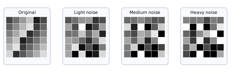
This is not a damaged photograph. It is a self-made small grid whose original signal and Gaussian noise are mixed with the weights in the equation. What matters is that a larger t leaves fewer original clues in the model input.
The Model Predicts Noise Rather Than a Finished Image
For training, choose an original x_0, a time step t, and noise epsilon, then construct x_t. The model receives x_t and t and predicts the noise that was added.
| Training step | What the model receives or makes | Why it is needed |
|---|---|---|
| 1 | original state x_0 | establishes a starting point from training data |
| 2 | time step t and noise epsilon | creates inputs with different noise levels |
| 3 | noisy state x_t | is the input the model actually reads |
| 4 | predicted noise epsilon_theta(x_t, t) | estimates what should be removed from the current state |
| 5 | difference between real and predicted noise | becomes the learning signal for loss and gradients |
In the simplest view, training reduces the mean squared error (MSE) between real and predicted noise.
This occupies the same place as the loss, gradient, and optimizer update loop earlier in Part 5. The new point is not a new kind of update: the target is the noise in the current step, rather than a class label or a completed image.
Reverse Generation Repeats from Noise
After training, we do not provide the original x_0. We begin with random noise, predict the current noise, and use that prediction to move to a slightly less noisy state. Repeating this creates a final state close to an image.
- Start from initial noise
x_T. - Give the current state
x_tand timetto the model and predict noise. - Use the scheduler rule to calculate the next state
x_(t-1). - Repeat until a generated state close to
x_0remains.
A scheduler is neither model weights nor a learning rate. It is the numerical rule that decides how to move from one generation state to the next using the model prediction. Thus the same trained model can follow a different restoration path when seed, steps, or scheduler changes.
| Value | Role to distinguish first |
|---|---|
| seed | reproduces the initial noise starting point |
| steps | number of reverse moves |
| scheduler | numerical rule for calculating the next state |
| model weights | learned values that predict noise or restoration direction |
Temperature, top-k, and top-p select among next-token candidates in text generation. A diffusion scheduler instead moves an image or latent state to its next restoration state. Both affect variation, but they are not the same algorithm.
Inspect a Small State Change
Keep the synthetic grid and its noise seed fixed, then change only the time step. The observation is not merely that heavy noise is hard to recognize. Changing t changes the model input x_t, and therefore changes the direction the model must estimate for removal.
| Change | Keep fixed | Observe |
|---|---|---|
time step t | original grid and noise seed | how original clues and noise weight change |
| noise seed | original grid and time step | how different noisy states are possible at one step |
| predicted-noise error | x_t and time step | how a smaller error improves the basis for the next move |
P6-21.3 handles a controlled test of a real public image model. Here it is enough to see diffusion as learning noise-removal directions at many levels and applying those predictions repeatedly, not as magic that directly retrieves an original image.
Checklist
- I can distinguish forward diffusion, noise-prediction training, and reverse generation.
- I can explain
x_0,epsilon,t, andx_t. - I can explain why the model learns to predict added noise instead of directly predicting a finished image.
- I can connect prediction error to the loss, gradient, and update flow in Part 5.
- I can distinguish a scheduler from model weights and from token sampling.
Sources and Further Reading
- Jonathan Ho, Ajay Jain, Pieter Abbeel, Denoising Diffusion Probabilistic Models, arXiv, 2020, accessed 2026-08-28.
- Yang Song et al., Score-Based Generative Modeling through Stochastic Differential Equations, arXiv, 2021, accessed 2026-08-28.